Intro to RStudio
Welcome to our RStudio Introduction! RStudio is a front end (user friendly) interface for R, a programming language for statistics. We’ll be using it to work with data and our various forms of functions.
RStudio is a long term learning goal for us. We will be adding new functions and learning new things throughout the semester.
Getting Started
Follow my lead as we get ourselves going with RStudio. We will
- Log in to RStudio
- Add some packages to the R environment
- Create a math135 directory to work in
- Create our first Rmd (‘R Markdown’) file
- Knit that Rmd file to create a PDF
You will need to replace the auto-generated code block at the top of your Rmd file with this one, which loads the mosaic functionality into the R environment when we knit to PDF.
```{r setup, include=FALSE, warning=FALSE}
knitr::opts_chunk$set(echo = TRUE)
suppressPackageStartupMessages(library(mosaic))
suppressPackageStartupMessages(library(mosaicCalc))
```
Pro Tip: Be kind to future you.
- Save all of your work for this class in the
math135subdirectory that we create today. - Give your files meaningful names. Include the unit, the topic, the date, etc, or a helpful combination of these identifiers.
R Markdown files
An R Markdown file is a hybrid file that has both text and code. You can then knit this Rmd file to make a lovely PDF.
Formatting Regular Text
The regular text uses Markdown, which has simple commands to create formatting such has sections, bold, italic, links, itemized lists, and much more. Here are is some example Markdown syntax.
# Heading

This is a regular sentence.

## Sub Heading

You get *italics like this.*

Skipping a line starts a new paragraph.
But if you don't skip a line then it's part of the same paragraph

### Sub Sub Heading

You get **bold text like this.**

Here is how to make an itemized list

* Make sure to skip a line before your first item
* The asterisk must be the **first** character on the line (no spaces!)
* If you want a sublist
   + Start the sublist on the line below the item
   + Indent by three spaces.
   + Use a plus sign
Here is a nice reference page for common R Markdown syntax.
Code Chunks
Your R code must be placed inside code chunks. Here is what a code chuck looks like
```{r}
1 + 1

sin(pi/4)
```
When you knit your Rmd file, the code chunks are executed in order. You can also run an individual chunk by clicking on the green arrow in its upper right corner.
Adding a code chunk is easy!
- In the top bar of the Markdown window, there’s a small, green plus C button.
- When you click this button, it’ll bring up options for code blocks to insert
- Select “R” which is the first option. (It’s the only one we will use.)
Writing Code
Add a code chunk and let’s get cracking!
Variables, Lists and Sequences
When we do a calculation, we can store the result for later. Here are some examples:
a = 15
b = 4 * a
R is particularly good at doing calculations on lists of data. So let’s make some lists!
RStudio makes a list with the c() command. The “c” in short for “combine”.
P=c(3, 5, 11, -1, 4)
P
## [1] 3 5 11 -1 4If you want to make a sequence, you use the seq() command. For example:
S=seq(1, 10)
S
## [1] 1 2 3 4 5 6 7 8 9 10Notice that the values increment by 1. You can use a different step size by adding a third argument. For exmaple, if I wanted a sequence 1, 1.1, 1.2, 1.3, etc… all the way up to 2, I would write
T=seq(1, 2, 0.1)
T
## [1] 1.0 1.1 1.2 1.3 1.4 1.5 1.6 1.7 1.8 1.9 2.0Now look at the Environment tab in the upper right window. What do you notice?
Pro Tips: Be kind to future you as well as current collaborators.
- Always write
0.1instead of.1in your code. It is much easier to read and to debug later! - Consider adding a space after your commas to separate parameters. It’s easier to read!
You Try
Try to do the following:
- Create a list
Xcontaining the values 8, 6, 7, 5, 3, 0, 9. - Create a list
Ycontaining the sequence of odd integers between (and including) 1 and 19 - What is the output of the command `X^2’? Can you see what R is doing?
- Try making another lists. Apply some functions to that list.
Functions
Now it’s time to write your own function. Here is how you create \(f(x)= x^2 -3\).
f = makeFun(x^2 - 3 ~ x)Much of this is pretty intuitive, except for maybe the final ~ x. This tilde symbol comes up a lot in RStudio and it indicates dependence. We need to tell RStudio that \(f\) is in terms of this variable \(x\), so it knows where to put an input when I ask it to.
Notice! In the right upper window, you now have a function called f. We can do a lot with this function, but
to start, let’s evaluate it at 1.
f(1)## [1] -2What do you think this code is doing?
S=seq(1, 10)
f(S)
## [1] -2 1 6 13 22 33 46 61 78 97Plotting
Let’s see how to create plots using RStudio. First, let’s create a plot of this data
| x | 0 | 1 | 2 | 3 | 4 | 5 |
| h(x) | 0 | 1 | 4 | 9 | 16 | 25 |
from the function \(h(x)=x^2\).
X = seq(0,5)
Y = X^2
gf_point(Y ~ X)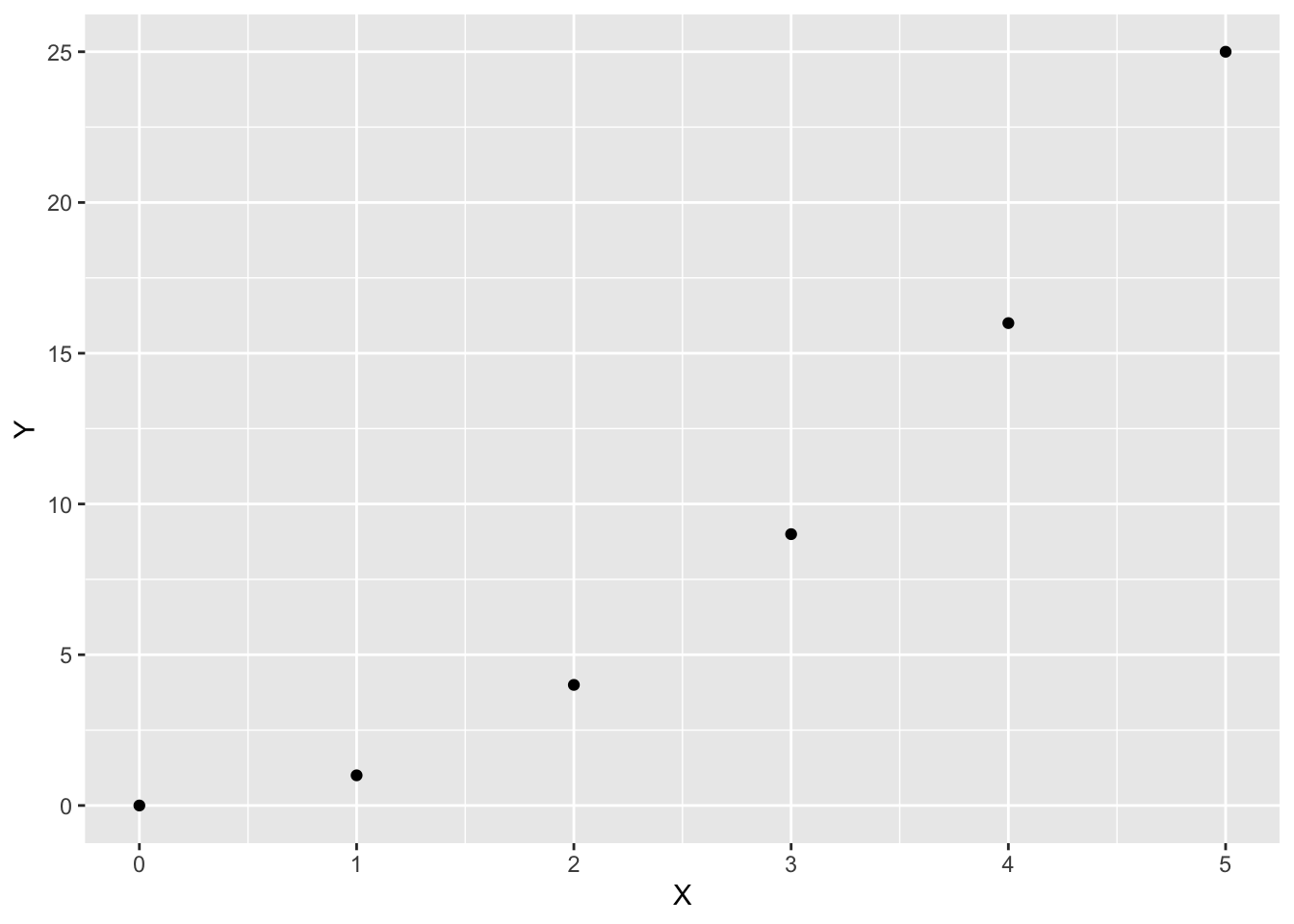
Notice! We list the dependent variable Y first and then the independent variable X after the tidle ~ (which matches the syntax of makeFun).
We can also plot a function. Once again the dependent variable appears after the tilde.
slice_plot(x^2 ~ x, domain(x=-2:2))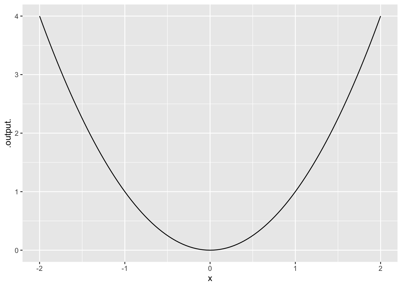
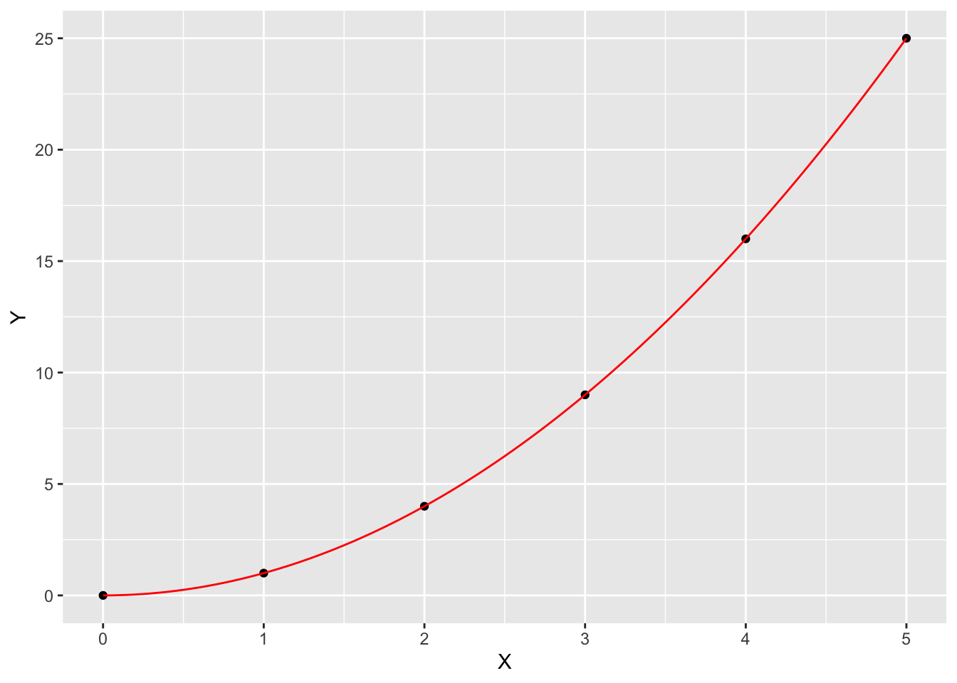
We can actually plot the data and the function on the same graph. We will plot the data and then add the function by using the add=TRUE parameter for plotFun. I will also use the optional col parameter to change the color of the function curve.
gf_point(Y ~ X) %>%
  slice_plot(x^2 ~ x, domain(x=0:5),color='red')