3.D Local Linear Approximation
The linearization of \(f(x)\) at \(x=a\) is \[ L_a(x) = f(a) + f'(a) (x-a). \]
The linearization of \(f(x,y)\) at point \((a,b)\) is \[ L_{(a,b)}(x,y) = f(a,b) + f_x(a,b) (x-a) + f_y(a,b) (x-b). \]
Activities
Estimating Sugar Solution Temperature
We are boiling a sugar solution to make salt water taffy. When we start, the temperature of the solution is \(80^\circ\)F, after 5 minutes it’s \(115^\circ\)F, and after 10 minutes it’s \(165^\circ\)F.
- Estimate the temperature after 17 minutes.
- The sugar solution needs to reach \(289^\circ\)F to be the consistancy of taffy. Estimate when this will happen.
Comparing Linearizations
- Draw two (nonlinear) functions \(f(x)\) and \(g(x)\) and their linearizations at \(x=1\). One function should be “well estimated” by the linearization around \(x=1\) and the other should be “poorly estimated” by the linearization around \(x=1\).
- What feature(s) of the curve \(y=f(x)\) result in a good approximation?
- What feature(s) of the curve \(y=g(x)\) result in a bad approximation?
Estimating a Function
Find the linearization \(L_2(x)\) the function \(g(t)=t^3+e^t-4\).
- Remember that \(L_2(x)\) means “the local linear approximation at \(x=2\).”
- You will need to use desmos to approximate \(f'(2)\).
- Remember that \(L_2(x)\) means “the local linear approximation at \(x=2\).”
Use your formula for \(L_2(x)\) to estimate \(g(2.1)\), \(g(1.98)\), \(g(3)\) and \(g(0.7)\).
Check your estimations with the original function.
What do you notice about your approximations as you get further from the spot where you built the linearization?
Estimating the Windchill
We’ve talked about windchill \(w(t,v)\) as a function of temperature \(t\) and wind speed \(v\). Here is the table that we’ve used
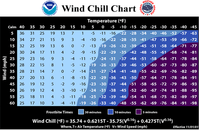
The perceived temperature when \(t=-10 ^\circ\)F and \(v=40\) mph is \(w(-10,40)=-43\). I have used desmos to estimate that \[ w_t(-10,-40) = 1.39, \qquad w_v(-10,40)= −0.28. \] Use these values to find the linearization \(L_{(-10,40)}(t,v)\) at the point \((-10,40)\).
Use your linearization (and desmos!) to estimate the four windchill values \(w(-5,40)\), \(w(-15,40)\), \(w(-10,45)\) and \(w(-10,35)\). Are your estimates close to the actual values?
Find the linearization of \(w(t,v)\) at \(t=-10\) and \(v=40\) using the the partial derivatives of the formula \(w(t,v) = 35.74+0.6215 t-35.75 v^{0.16}+0.4275 t \, v^{0.16}\). Here is a link to my desmos calculator for the partial derivatives of this function.
Solutions
Estimating Sugar Solution Temperature
Let’s use \(f(t)\) to denote the temperature.We need to estimate the rate of change at \(t=10\). We have \[ f'(10) \approx \frac{165 - 115}{10-5} = \frac{50}{5}=10\]. We use the linear approximation \[L_{10}(t) = 165 + 10 (t-10)\] to estimate the temperature. We have \[f(17) \approx L_{10}(17) = 165 + 10 (17-10) = 235.\]
We must solve \[ 289 = 165 + 10 (t-10) = 65t\] to find that \(10t = 224\) and so \(t=22.4\) minutes.
Comparing Linearizations
- In the graph below, the blue function is well estimated by its tangent line, while the red function is not.
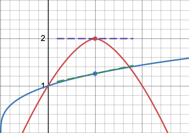
- If the curve has low concavity near the point \(x=a\) then the tangent line is a good approximation. In other words, the second derivative remains near zero around the point \(x=a\)
- If the curve has a lot of concavity near the point \(x=a\) then then tangent line is not a good approximation. This is because the curve bends away from the tangent line.
Estimating a Function
Using desmos, I found that \(f(2)=11.39\) and \(f'(2)=19.39\). Therefore \[ L_2(t) = 11.39 + 19.39 ( t-2).\]
I get the estimates \(g(2.1) \approx 13.33\), \(g(1.98) \approx 11.00\), \(g(3) \approx 30.78\) and \(g(0.7) \approx -13.82\).
The true values are \(g(2.1) = 13.43\), \(g(1.98) = 11.01\), \(g(3) = 43.09\) and \(g(0.7) \approx -1.64\)..
The approximations close to \(t=2\) are much better!
Estimating the Windchill
\(L_{(-10,40)}(t,v) = -43 + 1.39(t+10) -0.24(v-40)\)
My estimates are \(w(-5,40) \approx -36.05\), \(w(-15,40) \approx -49.95\), \(w(-10,45) \approx 41.8\) and \(w(-10,35) \approx -44.2\). These are pretty close to the values on the table.
Using the function and the partial derivatives from this desmos calculation, we get \[ L_{(-10,40)}(t,v) = -42.70 + 1.39(t+10) -0.29(v-40) \]