5.B 2D Optimization

Summary

The critical points of $f(x,y)$ are the points $(a,b)$ where both $f_x(a,b)=0$ and $f_y(a,b)=0$.

There are three ways to determine whether a critical point $(a,b)$ is a minimum, a maximum, or a saddle point.

Find the values of $f(a,b) - f(x,y)$ for points $(x,y)$ in a small circle around $(a,b)$.
- If these values are ALL positive then $(a,b)$ is a local maximum
- If these values are ALL negative then $(a,b)$ is a local minimum
- If some values are positive and some values are negative, then $(a,b)$ is a saddle point.
Create a contour plot for $f(x,y)$ on a very small neighborhood of $(a,b)$. Use the contours to figure out whether it is a local max, a local min, or a saddle point.
The second derivative test relies on the value \[ D = f_{xx} f_{yy} - (f_{xy})^2. \]
- If $D > 0$ and $f_{xx} > 0$ then $(a,b)$ is a local minimum.
- If $D > 0$ and $f_{xx} < 0$ then $(a,b)$ is a local maximum
- If $D < 0$ then $(a,b)$ is a saddle point
- If $D=0$ then the test fails

Among these options, #1 is the easiest to use. Here is a link to a desmos workbook that classifies the critical point $(2,-1)$ of the function $f(x,y)= x^2+ 2y^4+ 4xy$ by creating a table of values $f(2,1) - f(c,d)$ where the points $(c,d)$ are in a small circle around $(2,1)$.

Here is some R code that does the same thing.

f = makeFun(x^2 + 2*y^4 + 4*x*y ~ x&y)
a=2
b=-1

r = 0.1
theta = seq(0,2*pi,pi/10)
f(a,b) - f(a+r*cos(theta), b+r*sin(theta))

##  [1] -0.010000000 -0.032025526 -0.065424470 -0.096866673
##  [5] -0.114533357 -0.112200000 -0.091021947 -0.058824413
##  [9] -0.027382209 -0.008514116 -0.010000000 -0.032497662
## [13] -0.068673667 -0.105338809 -0.128297176 -0.128200000
## [17] -0.104785766 -0.067296549 -0.030631406 -0.008986252
## [21] -0.010000000

All of the values are negative, which means that $f(2,-1)$ is a local minimum.

Activities

Characterize the Extrema

Multiple 2D functions have been (contour) plotted below. For each, identify the critical points and determine if they are maximums, minimums, or saddle points.

f = makeFun(x^2+y^2+3~x&y)
contour_plot(f(x,y)~x&y, domain(x=-2:2, y=-2:2), skip = 0)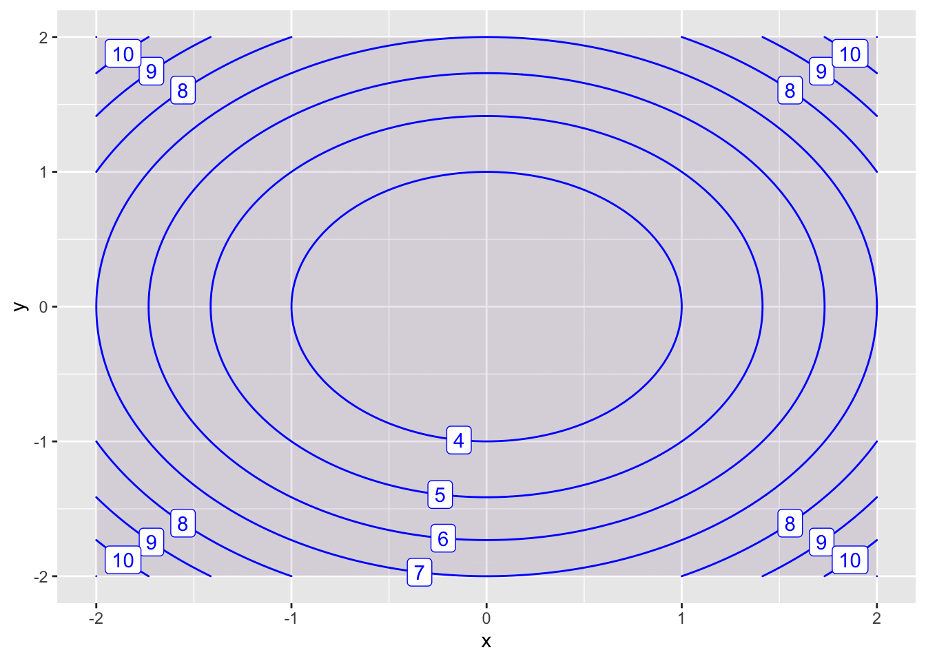

f = makeFun(-x*y*exp(-x^2-y^2)~x&y)
contour_plot(f(x,y)~x&y, domain(x=-1.5:1.5, y=-1.5:1.5), skip = 0)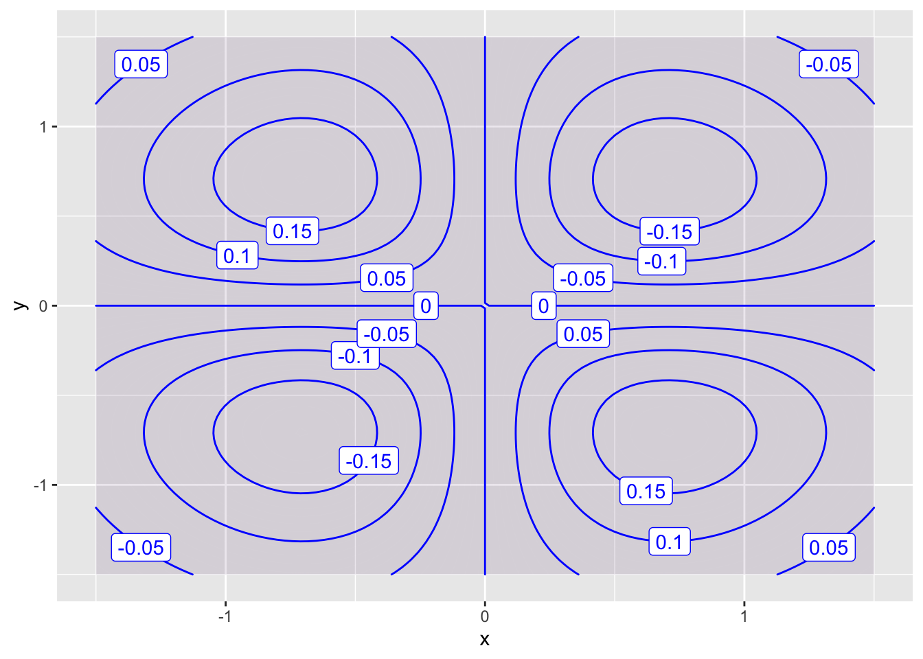

f = makeFun(y^2-x^2~x&y)
contour_plot(f(x,y)~x&y, domain(x=-2:2, y=-2:2), skip = 0)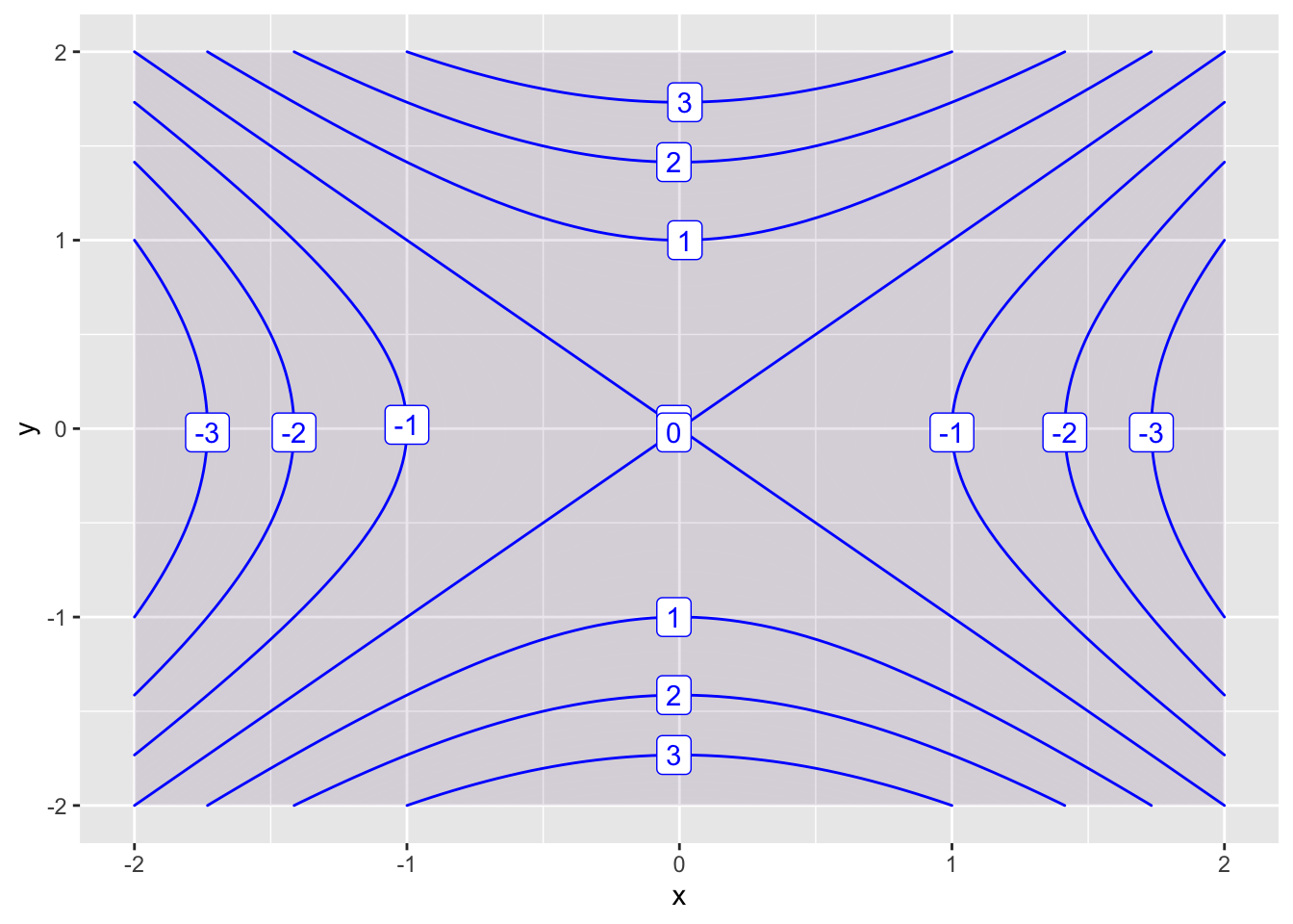

f = makeFun(cos(x)*(x^2-y^2)~x&y)
contour_plot(f(x,y)~x&y, domain(x=-1.5:1.5, y=-1.5:1.5), skip = 1)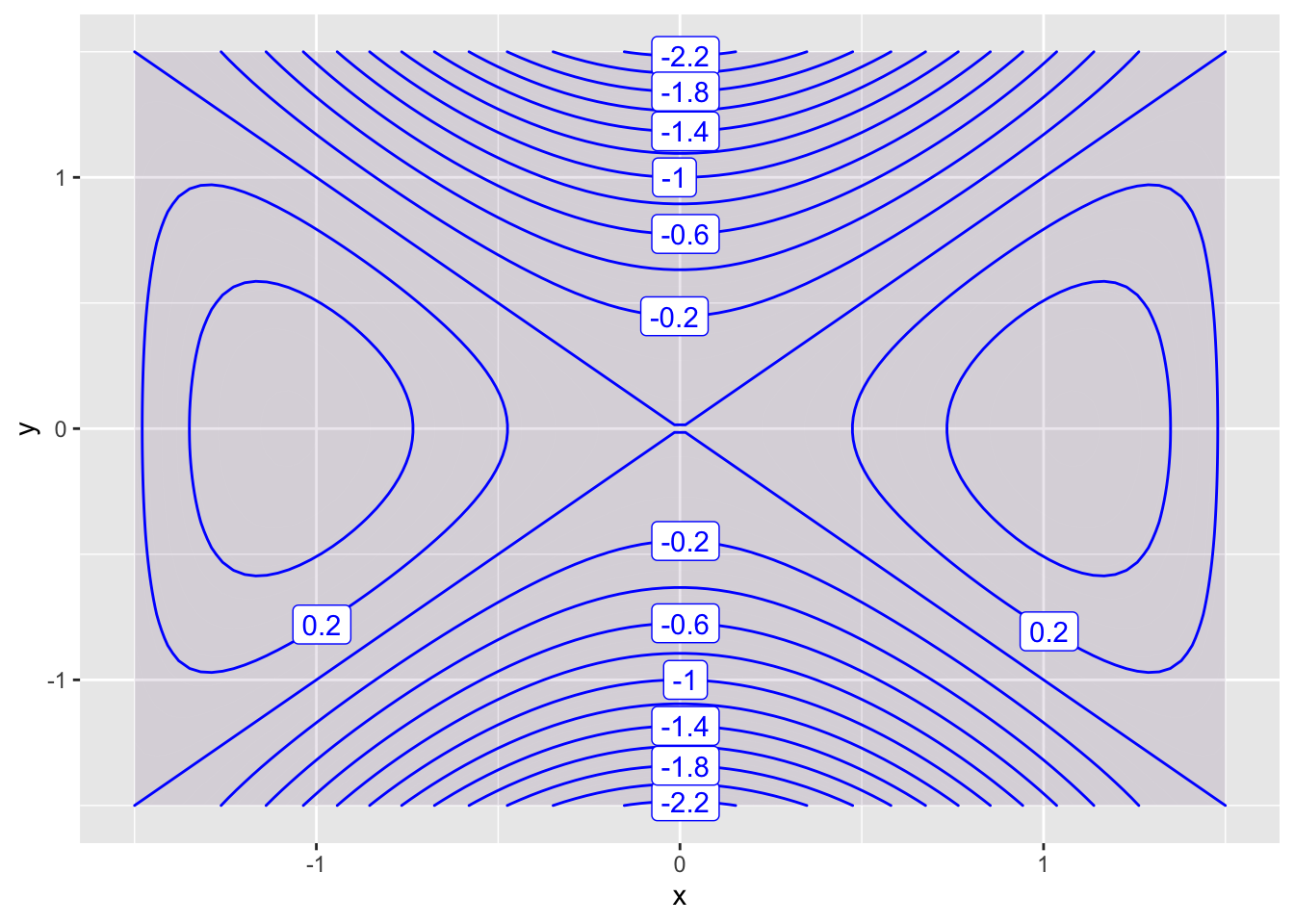

Classifying a critical point using a small circle of values

The function $f(x,y) =3x^2y + y^3 -3x^2-3y^2+3$ has four critical points: \[ (0,0) \qquad (0,2) \qquad (1,1) \qquad (1,,-1). \] For each critical point $(a,b)$, evaluate $f(a,b) - f(x,y)$ in a small circle centered at $(a,b)$ to determine whether it is a local minimum, a local maximum, or a saddle point

The 2D Second Derivative Test

The function $f(x,y)=10 + x^3 + 8y^3 - 3xy$ has two critical points: $(0,0)$ and $(1/2,1/4)$.

Use the second derivative test to classify each point as a local minimum, local maximum, or saddle point. For convenience, here are the second derivatives of $f(x,y)$.

\[ f_{xx} = 6x, \qquad f_{yy} = 48y, \qquad f_{xy} = -3. \]

Confirm that your answer is correct by creating a contour plot on a very small neighborhood around each critical point.

Classify the Critical Points

Find the critical points of $f(x,y)=9-2x+4y-x^2-4y^2$. Then use any method that you like to classify each one as a local minimum, a local maximum or a saddle point.

Optimizing Flight Control

The range over which a flying drone can be guided is related to the atmospheric temperature and humidity. The range function is \[ R(t,h)=27800-5t^2-6ht-3h^2+400t+300h \] What are the optimal atmospheric conditions?

Solutions

Characterize the Extrema

Plot 1 * Local minimum at $(0,0)$

Plot 2 * Local minima at $(-0.75, -0.75)$ and $(0.75, 0.75)$ * Local maxima at $(-0.75, 0.75)$ and $(0.75, -0.75)$ * Saddle point at $(0,0)$

Plot 3 * Saddle point at $(0,0)$

Plot 4 * Local maxima at $(-1,0)$ and $(1,0)$ * Saddle point at $(0,0)$

Classifying a critical point using a small circle of values

Let’s define our function and then check each of our critical points.

f = makeFun(3*x^2*y + y^3 -3*x^2-3*y^2+3~x&y)

First, we check $(0,0)$ and find that it is a local maximum.

a=0
b=0
r = 0.1
theta = seq(0,2*pi,pi/10)
f(a,b) - f(a+r*cos(theta), b+r*sin(theta))

##  [1] 0.03000000 0.02913197 0.02864279 0.02863197 0.02886731
##  [6] 0.02900000 0.02886731 0.02863197 0.02864279 0.02913197
## [11] 0.03000000 0.03086803 0.03135721 0.03136803 0.03113269
## [16] 0.03100000 0.03113269 0.03136803 0.03135721 0.03086803
## [21] 0.03000000

Next, we check $(0,2)$ and find that it is also a local minimum.

a=0
b=2
r = 0.1
theta = seq(0,2*pi,pi/10)
f(a,b) - f(a+r*cos(theta), b+r*sin(theta))

##  [1] -0.03000000 -0.03086803 -0.03135721 -0.03136803 -0.03113269
##  [6] -0.03100000 -0.03113269 -0.03136803 -0.03135721 -0.03086803
## [11] -0.03000000 -0.02913197 -0.02864279 -0.02863197 -0.02886731
## [16] -0.02900000 -0.02886731 -0.02863197 -0.02864279 -0.02913197
## [21] -0.03000000

Next up is $(1,1)$.It is a saddle point!

a=1
b=1
r = 0.1
theta = seq(0,2*pi,pi/10)
f(a,b) - f(a+r*cos(theta), b+r*sin(theta))

##  [1]  0.00000000 -0.01850159 -0.02988890 -0.02989973 -0.01876625
##  [6] -0.00100000  0.01650087  0.02716366  0.02717449  0.01676552
## [11]  0.00000000 -0.01676552 -0.02717449 -0.02716366 -0.01650087
## [16]  0.00100000  0.01876625  0.02989973  0.02988890  0.01850159
## [21]  0.00000000

One more point to go: $(1,-1)$. This is also a saddle point.

a=1
b=-1
r = 0.1
theta = seq(0,2*pi,pi/10)
f(a,b) - f(a+r*cos(theta), b+r*sin(theta))

##  [1]  1.2600000  0.8119458  0.2955892 -0.2353778 -0.7292137
##  [6] -1.1410000 -1.4355873 -1.5889990 -1.5889882 -1.4353227
## [11] -1.1400000 -0.7272129 -0.2326526  0.2983144  0.8139466
## [16]  1.2610000  1.5908545  1.7660624  1.7660516  1.5905898
## [21]  1.2600000

The 2D Second Derivative Test

The function $f(x,y)=10 + x^3 + 8y^3 - 3xy$ has two critical points: $(0,0)$ and $(1/2,1/4)$.

The critical points are $(0,0)$ and $(1/2,1/4)$. The second derivatives are \[ f_{xx} = 6x, \qquad f_{yy} = 48y, \qquad f_{xy} = -3. \] so our second derivative test function is \[ D(x,y) = (6x)(48y) - 9. \] We have $D(0,0) = -9$ so $(0,0)$ is a saddle point. We have $D(1/2,1/4)= 3 \cdot 12 - 99 = 36 - 9 > 0$. So we further check that $f_{xx}(1/2,1/4) = 3 > 0$ which means that $(1/2, 1/4) is a local minimum.
Here is a plot that shows that $(0,0)$ is a saddle point.

f = makeFun(10 + x^3 + 8*y^3 - 3*x*y~x&y)
contour_plot(f(x,y)~x&y, domain(x=-1:1, y=-1:1), skip=0)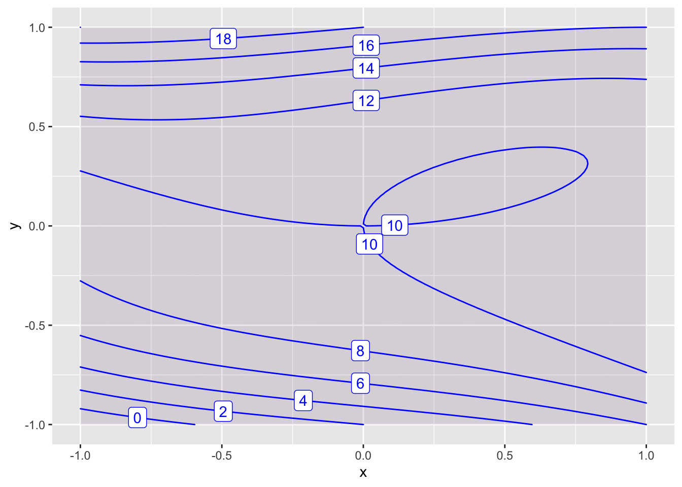

Here is another plot that zooms in on $(1/2,1/4)$. It is clear that this is a local minimum.

f = makeFun(10 + x^3 + 8*y^3 - 3*x*y~x&y)
contour_plot(f(x,y)~x&y, domain(x=0:1, y=0:1), skip = 0)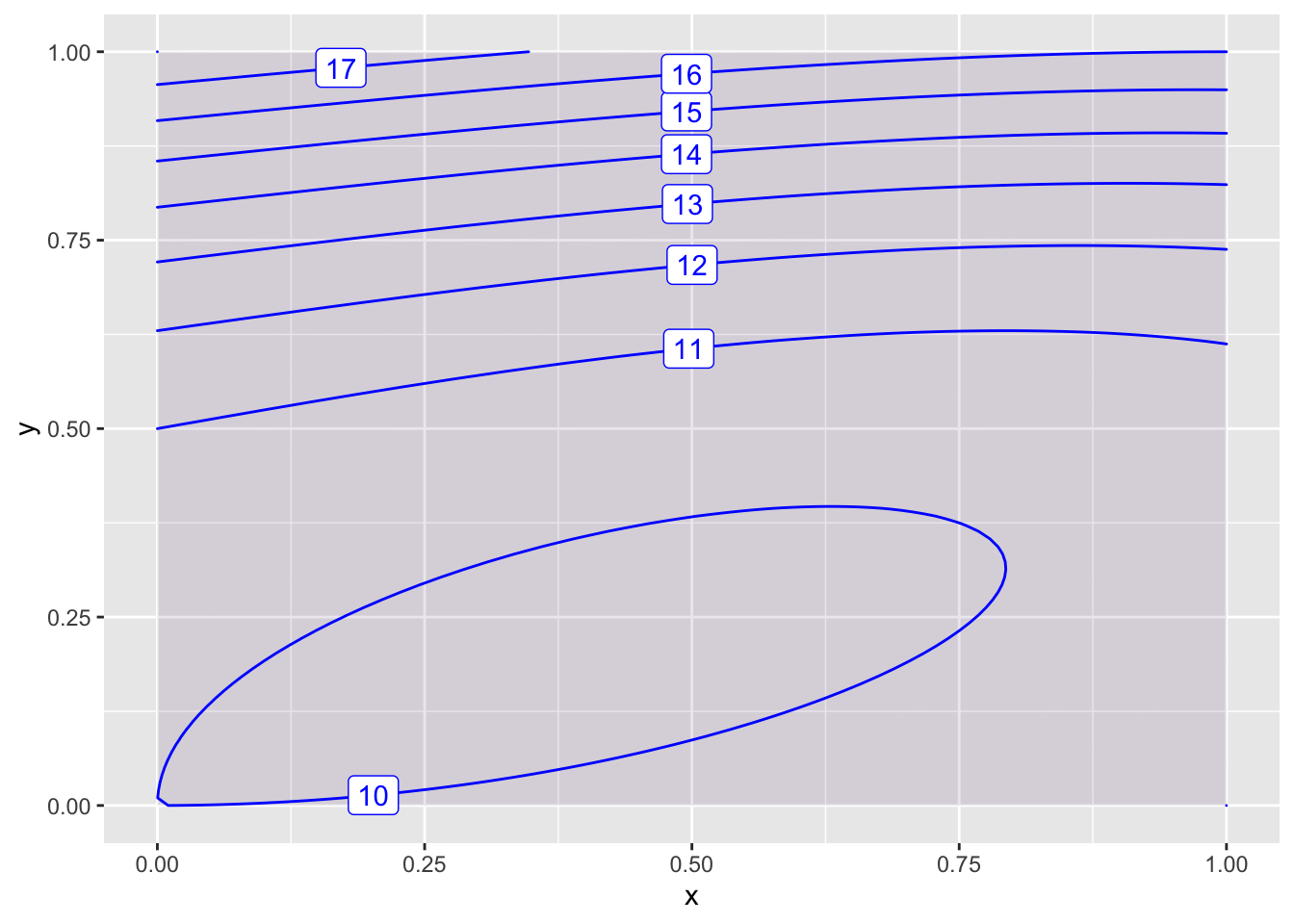

Classify the Critical Points

Let’s find the critical points of $f(x,y)=9-2x+4y-x^2-4y^2$. We have \[ f_x(x,y) = -2-2x, \qquad f_y(x,y) = 4 - 8y. \]

The only critical point is $(-1, 1/2)$. Let’s compare $f(-1,1/2)$ to the values of $f(x,y)$ on a small circle around this point.

f=makeFun(9 - 2*x + 4*y - x^2 - 4*y^2 ~ x&y)
a=-1
b=1/2
r = 0.1
theta = seq(0,2*pi,pi/10)
f(a,b) - f(a+r*cos(theta), b+r*sin(theta))

##  [1] 0.01000000 0.01286475 0.02036475 0.02963525 0.03713525
##  [6] 0.04000000 0.03713525 0.02963525 0.02036475 0.01286475
## [11] 0.01000000 0.01286475 0.02036475 0.02963525 0.03713525
## [16] 0.04000000 0.03713525 0.02963525 0.02036475 0.01286475
## [21] 0.01000000

This is a local maximum!

Optimizing Flight Control

Our function is $R(t,h)=27800-5t^2-6ht-3h^2+400t+300h$. Our partial derivatives are \[ \begin{array}{rcl} f_t(t,h) &=& -10t - 6h + 400 \\ f_h(t,h) &=& -6t-6h+300 \end{array} \] Setting both to zero, \[ \begin{array}{rcl} -10t - 6h + 400 &=& 0\\ -6t-6h+300 &=& 0 \end{array} \] we subtract the second from the first to find that $-4t+100 = 0$ and so $t=25$. This means that $-250 - 6h +400 = 0$ which becomes $6h = 150$ and therefore $h = 25$. So the optimal conditions are $t=25$ and $h=25$.