5.D Constrained 2D Optimization
Creating a Contour Plot for 2D Optimization
Here is some example code to create a plot of an objective function \(P(x,y) = x^{0.2} y^{0.8}\) and a constraint function \(Q(x,y)=4x + 3y=200\).
P = makeFun( x^(0.2) * y^(0.8) ~ x&y)
Q = makeFun( 4*x + 3*y ~ x&y)

contour_plot(P(x,y)~x&y, domain(x=0:40, y=20:80),
             contours_at=seq(20,70,6), skip=0) |>
  contour_plot(Q(x,y) ~ x & y, contour_color="black",
               contours_at=c(200), label_placement=.25)
## Scale for 'colour' is already present. Adding another scale for
## 'colour', which will replace the existing scale.## Scale for 'fill' is already present. Adding another scale for
## 'fill', which will replace the existing scale.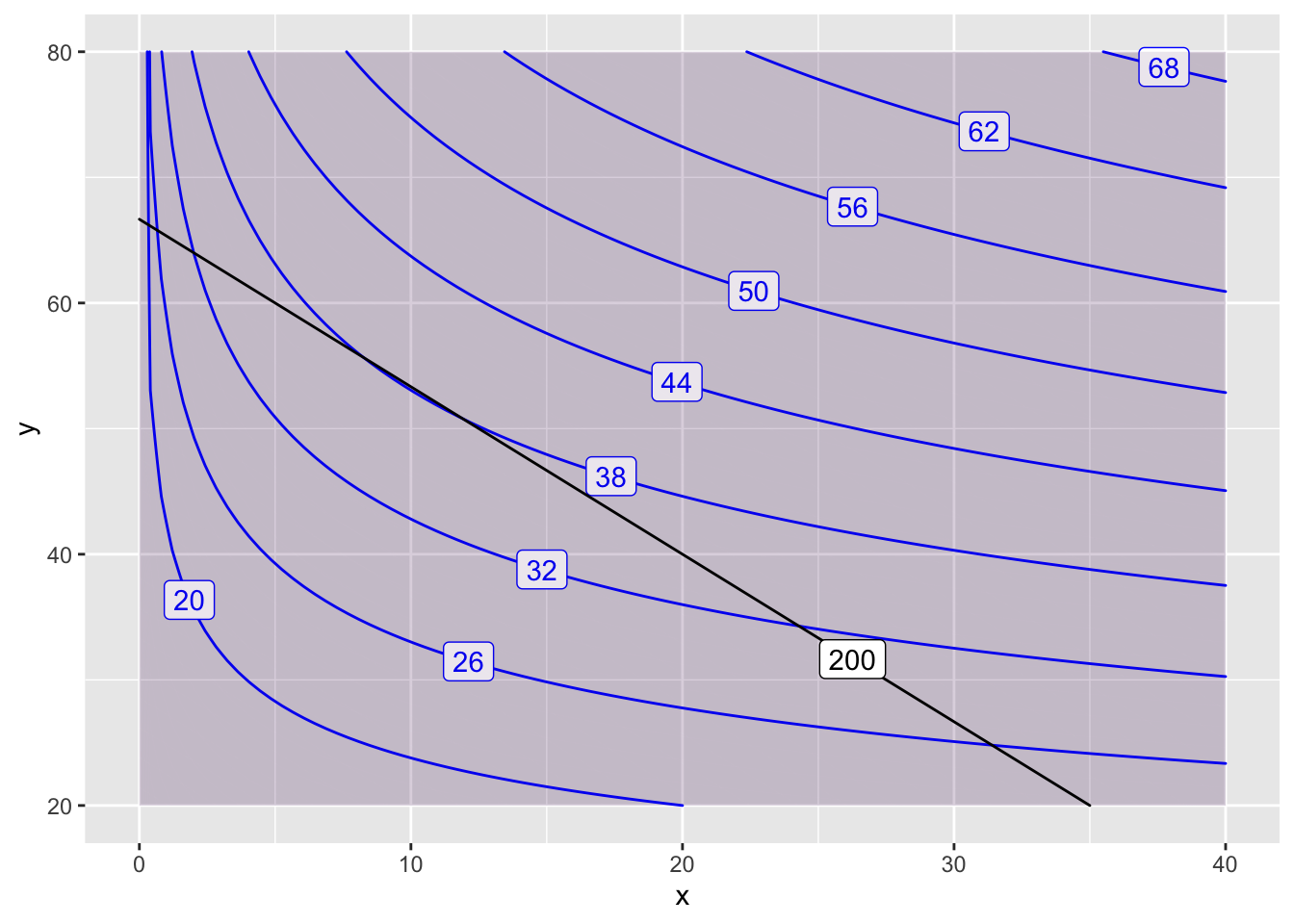
Activities
Constrained Production
A company produces \(P(x,y) = 100 x^{4/11} y^{7/11}\) units of its product from raw materials \(x\) and \(y\). The cost of each unit of \(x\) is $5 and the cost of each unit of \(y\) is $4.
Find the maximal output for a budget of $500, along with how much input \(x\) and \(y\) is used to create them. (Hint: plot your contour diagram on the domain \(0 \leq x \leq 100\) and \(0 \leq y \leq 100\). Start with the default contours by removing the
levelsinput.)What is the maximal output if the unit cost of \(x\) increases to $7? How much of inputs \(x\) and \(y\) are used?
What is the maximal output if the unit cost of \(x\) returns to $5 and the budget is decreased to $300? How much of inputs \(x\) and \(y\) are used?
Constrained Optimization on a Circle
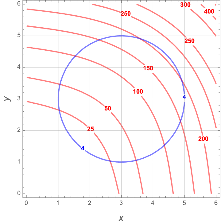
Below is a plot of an objective function \(f(x,y)\) in red, and its constraint function \(g(x,y)=4\) in blue.
- Estimate the minimum value of \(f(x,y)\) constrained to \(g(x,y)=4\). What point achieves this minimum?
- Estimate the maximum value of \(f(x,y)\) constrained to \(g(x,y)=4\). What point achieves this maximum?
Estimating the Lagrange Multiplier
Below is a plot of an objective function \(f(x,y)\) in red, and its constraint function \(g(x,y)\) for various budgets in blue (in thousands of dollars).
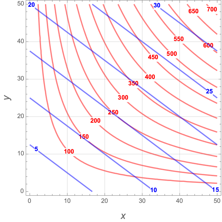
- Estimate the point \((x,y)\) that maximizes production for a budget of \(g(x,y)=15\). What is the production level?
- Estimate the point \((x,y)\) that maximizes production for a budget of \(g(x,y)=20\). What is the production level?
- What is the value of the Lagrange multiplier for the budget \(g(x,y)=15\)? What are the units? What does this number mean?
- What price would make this increase useful to the company? (Hint: the units for your answer are “dollars per unit produced.”)
Solutions
Constrained Production
- Here is our plot of the objective function \(P(x,y)\) and the constraint \(Q(x,y) = 500\).
P = makeFun( x^(4/11) * y^(7/11) ~ x&y)
Q = makeFun( 5*x + 4*y ~ x&y)

contour_plot(P(x,y)~x&y, domain(x=0:100, y=0:100), skip=0) |>
  contour_plot(Q(x,y) ~ x & y, contour_color="black",
               contours_at=c(500), label_placement=.25)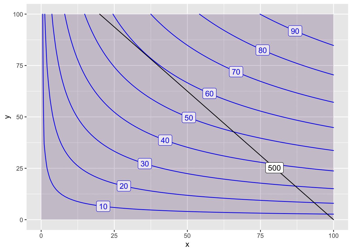
The maximum output for our budget occurs where the \(Q(x,y)=500\) constraint is tangent to a contour of \(P(x,y)\). This occurs at (approximately) the point \((38,78)\) and we estimate that the maximum production is \(P(38,78)=60\).
- We need to make a new plot using an updated objective function.
P = makeFun( x^(4/11) * y^(7/11) ~ x&y)
Q = makeFun( 7*x + 4*y ~ x&y)

contour_plot(P(x,y)~x&y, domain(x=0:100, y=0:100), skip=0) |>
  contour_plot(Q(x,y) ~ x & y, contour_color="black",
               contours_at=c(500), label_placement=.25)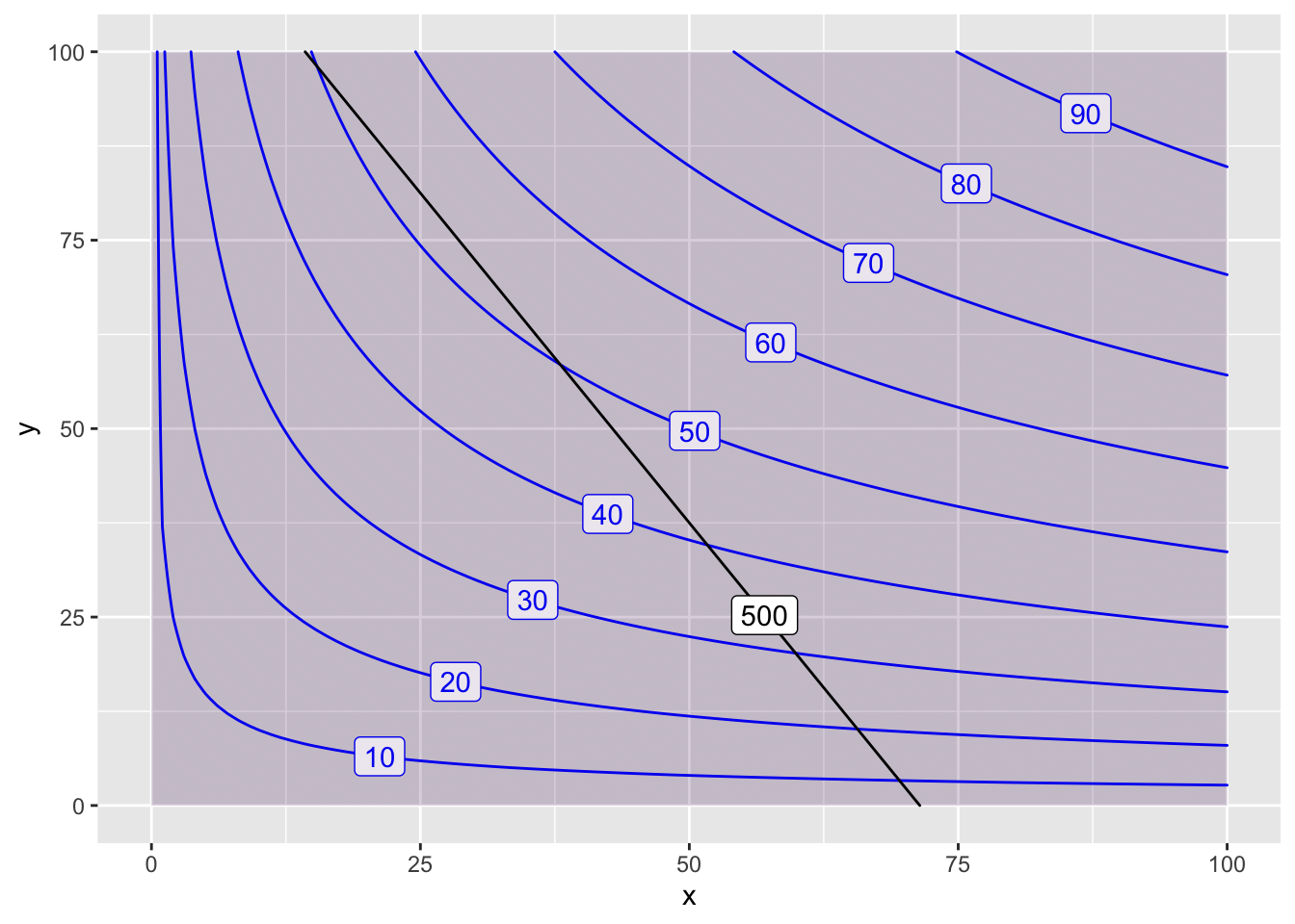
Now, the constraint isn’t tangent to any of the shown contours, but it IS tangent to a contour that we haven’t drawn! That point is somewhere around (25, 80), and the optimal productions probably around 52 or so. Let’s make another plot on a smaller domain and pick some contours to draw.
contour_plot(P(x,y)~x&y, domain(x=0:50, y=50:100), skip=0,
             contours_at = seq(23,73,5)) |>
  contour_plot(Q(x,y) ~ x & y, contour_color="black",
               contours_at=c(500), label_placement=.25)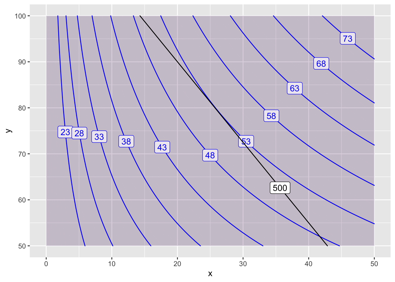
After some experimentation, I realized that \(P(x,y)=53\) is the contour that is tangent \(Q(x,y)=500\). So the optimal point is \((26,80)\) and the optimal output is 53.
- Now we return to the original constraint function, but decrease the budget to \(300\).
P = makeFun( x^(4/11) * y^(7/11) ~ x&y)
Q = makeFun( 7*x + 4*y ~ x&y)

contour_plot(P(x,y)~x&y, domain(x=0:50, y=25:75), skip=0) |>
  contour_plot(Q(x,y) ~ x & y, contour_color="black",
               contours_at=c(300), label_placement=.25)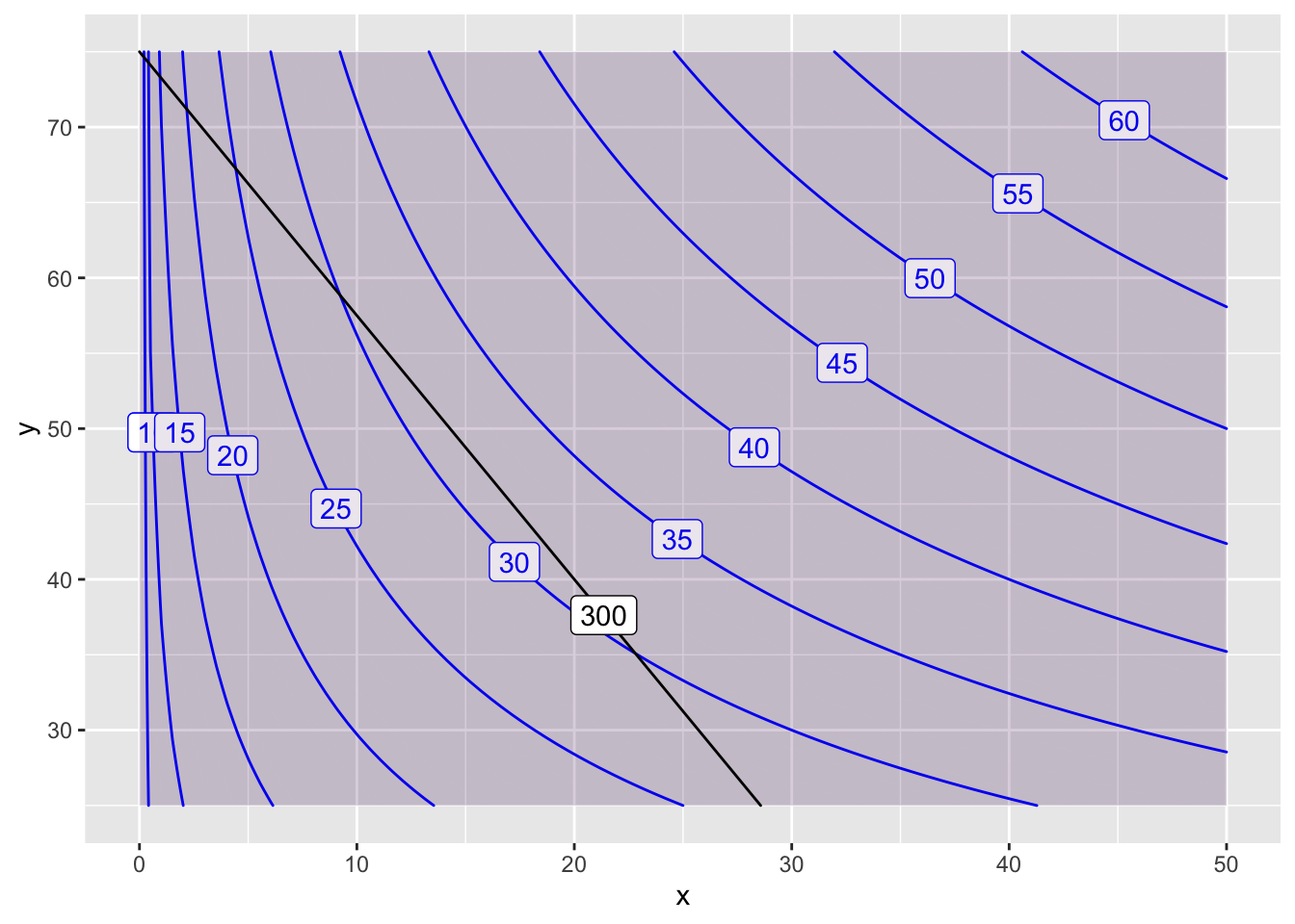
The optimal point is at \((21,40)\) and the optimal production is approximately \(f(21,40)=32\).
Constrained Optimization on a Circle
- The minimum is approximately \(f(1.5, 1.5) = 20\).
- The maximum is approximately \(f(4.5, 4.5) = 210\).
Estimating the Lagrange Multiplier
For a budget of 15, the maximal production is \(f(25,18)=250\).
For a budget of 20, the maximal production is \(f(32,26)=360\).
The Lagrange multiplier is \[ \lambda = \frac{\triangle \mbox{production}}{\triangle \mbox{constraint}} \approx \frac{360-250}{20-15}=\frac{110}{5}=22 \frac{\mbox{units}}{\mbox{dollar}} \] So if we increase our budget by $1, then we will produce 22 more units.
The Lagrange multiplier is approximately \(22\) units/dollar. We will break even if we can sell one unit for \(1/22=0.045\) dollars/unit. So if the sale price is at least $0.045, we will decide to increase production.