7.D Slope Fields

Creating a Slope Field in RStudio

The mosaicCalc package has a vectorfield_plot function that we use to create a slope field. So we need to make sure that this package has been loaded into RStudio.

suppressPackageStartupMessages(library(mosaicCalc))

Here is the code to create the slope field for \(\displaystyle{\frac{dP}{dt} = 6 - 2 P}\)

vectorfield_plot(t ~ 1,
P ~ 6 - 2 * P,
domain(t=-8:8, P=-8:8))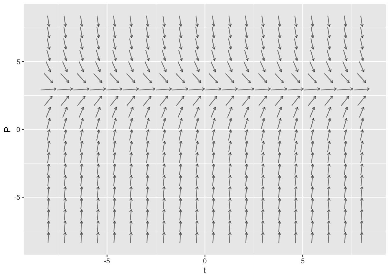

Creating a Trajectory in RStudio

The mosaicCalc package also has a traj_plot function that plots a solution curve to a differential equation through a given initial point.

Here is the code to plot the trajectory starting at \(P(0)=6\) for the differential equation \(\displaystyle{\frac{dP}{dt} = 6 - 2 P}\). In the code below, the nt parameter indicated the number of “tick marks” to use along the trajectory.

dyn = makeODE( dP ~  6 - 2 * P )
soln = integrateODE(dyn, domain(t=0:5), P=6)
traj_plot(P(t) ~ t, soln,  nt=5)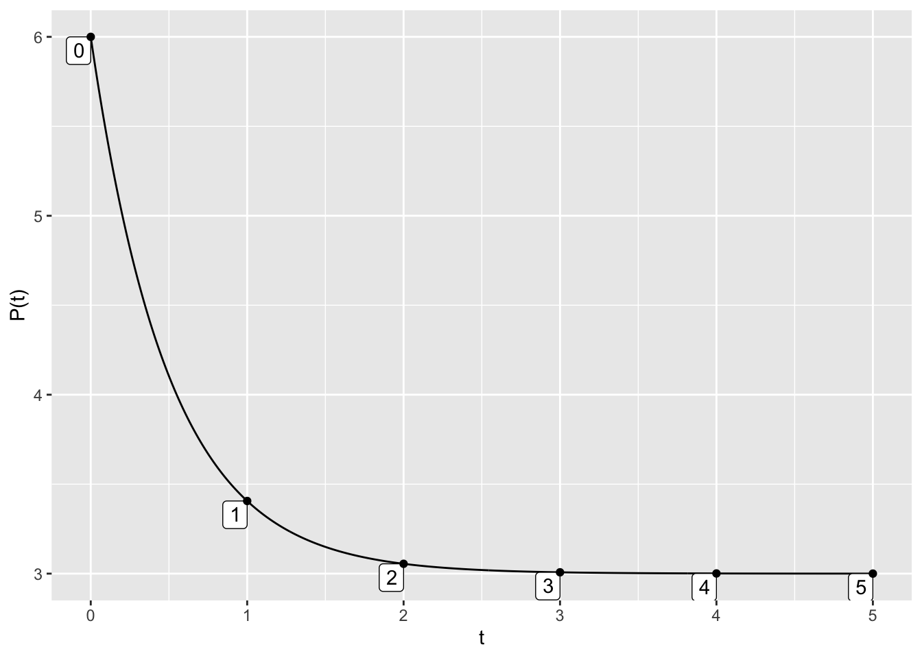

In fact, we can get fancier by making a single plot that has two trajectories (one for \(P(0)=6\) and one for \(P(0)=2\)) along with the vector field.

dyn = makeODE( dP ~  6 - 2 * P )
soln1 = integrateODE(dyn, domain(t=0:5), P=6)
soln2 = integrateODE(dyn, domain(t=0:5), P=2)
traj_plot(P(t) ~ t, soln1, color="blue", nt=0) %>%
  traj_plot(P(t) ~ t, soln2, color="magenta", nt=0) %>%
  vectorfield_plot(t ~ 1, P ~ 6 - 2 * P, domain(t=0:5, P=0:8))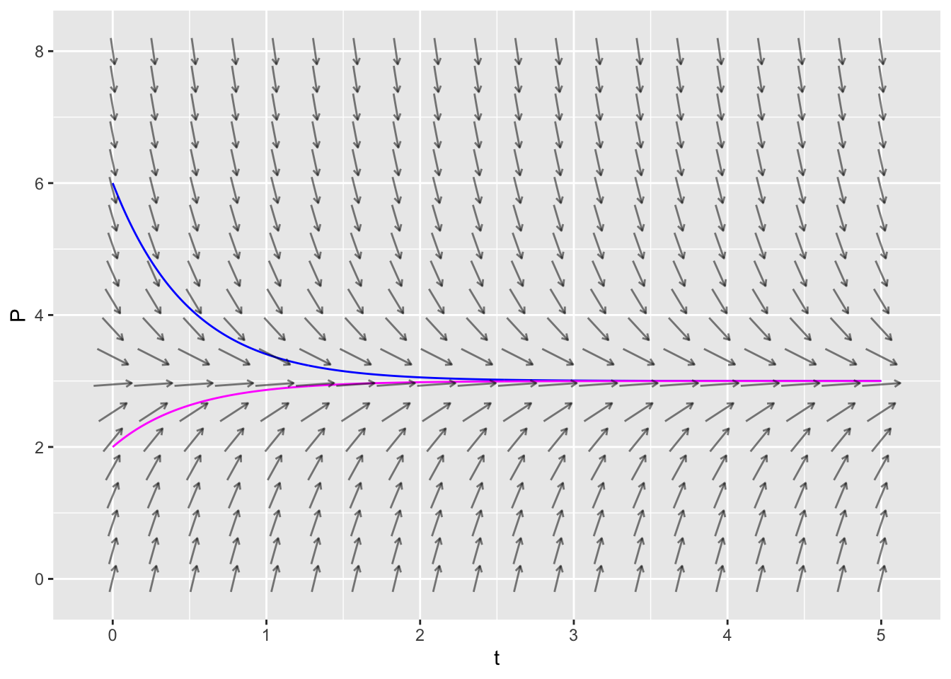

Activities

Match the Slope Field

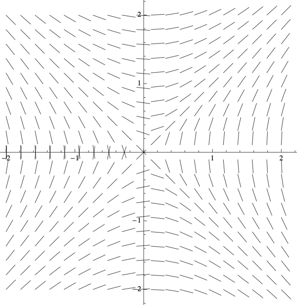
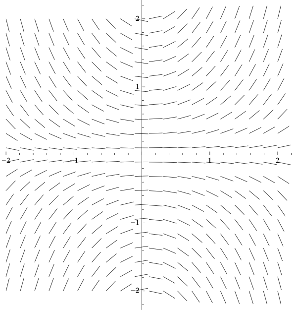
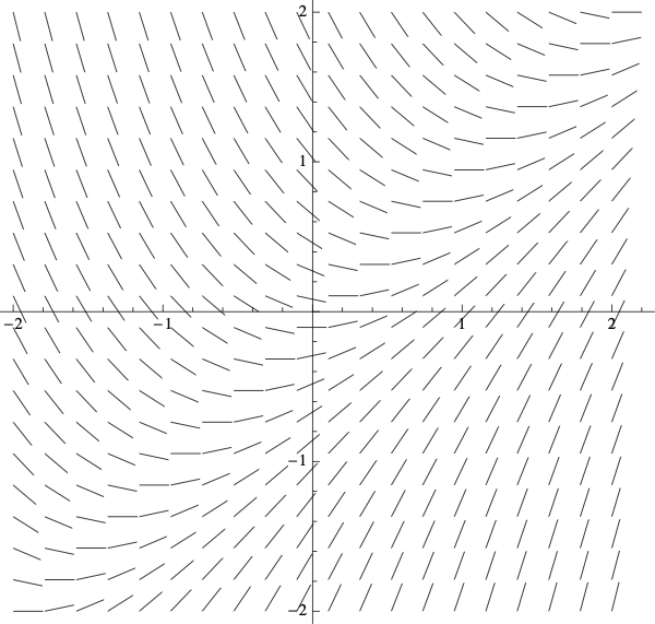
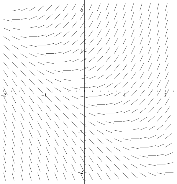
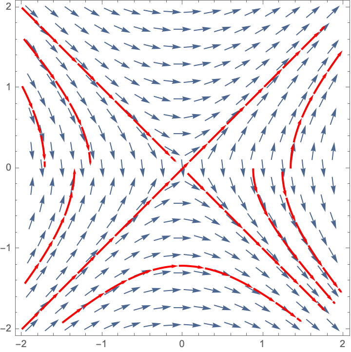
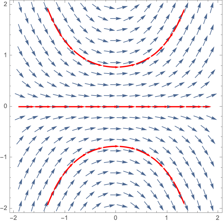
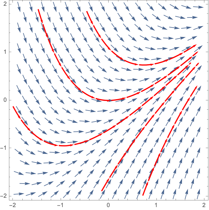
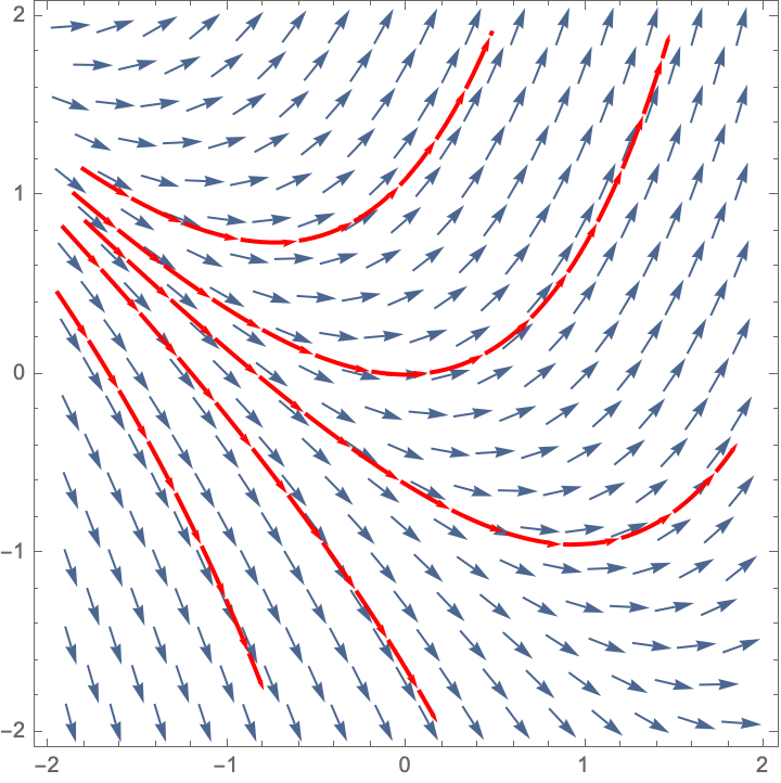
Match each of the following differential equations with its slope field. Hint: start by setting \(\frac{dy}{dx} = 0\) and solving for \(y\). The slopes along the resulting curve will always be horizontal.

\(\displaystyle{\frac{dy}{dx}=xy}\)
\(\displaystyle{\frac{dy}{dx}=\frac{x}{y}}\)
\(\displaystyle{\frac{dy}{dx}=x+y}\)
\(\displaystyle{\frac{dy}{dx}=x-y}\)

Slope Field A	Slope Field B


Slope Field C	Slope Field D

Draw Some Trajectories

For each of the above slope fields, sketch the solution curves that satisfy

\(y(0) = 1\)
\(y(0) = 0\)
\(y(0) = -1\)

Removing a Pollutant

A pollutant spilled on the ground decays at a rate of 4% a day. In addition, cleanup crews remove the pollutant at a rate of 20 gallons a day.

Write a differential equation for the amount of pollutant \(P\), in gallons, left after \(t\) days.
The initial amount of pollutant is 2000 gallons. Use the plot_traj command to create a trajectory for \(0 \leq t \leq 50\). Set nt=10 to show 10 tick marks on your trajectory.
Use the trajectory to estimate long it takes to clean up the pollutant. In other words, when is \(P(t)=0\)?

Slope Fields for Population Models

Create a slope field for each of the following population models. For each one, describe the long-term behavior for a variety of intial populations. For which initial values of \(P\) does the population increase without bound? stabilize to a constant value? die out?

Exponential growth with harvesting. \[ \frac{dP}{dt} = 0.2 P - 40 \] for \(0 \leq P \leq 300\) and \(0 \leq t \leq 100\).
Constrained growth \[ \frac{dP}{dt} = 0.05 P (1 - 0.002 P) \] for \(0 \leq P \leq 600\) and \(0 \leq t \leq 50\).
Constrained growth with constant harvesting \[ \frac{dP}{dt} = 0.05 P (1 - 0.002 P) - 4 \] for \(0 \leq P \leq 600\) and \(0 \leq t \leq 50\).

Trajectories for Population Models

Now create trajectories for the population models in the previous exercise. Create a trajectory for each of the different possible outcomes (increase without bound, stabilize to a constant value, die out)

Exponential growth with harvesting. \[ \frac{dP}{dt} = 0.2 P - 40 \] for \(0 \leq P \leq 300\) and \(0 \leq t \leq 100\).
Constrained growth \[ \frac{dP}{dt} = 0.05 P (1 - 0.002 P) \] for \(0 \leq P \leq 600\) and \(0 \leq t \leq 50\).
Constrained growth with constant harvesting \[ \frac{dP}{dt} = 0.05 P (1 - 0.002 P) - 4 \] for \(0 \leq P \leq 600\) and \(0 \leq t \leq 50\).

Solutions

Match the Slope Fields

\(\displaystyle{\frac{dy}{dx}=xy}\) is Slope Field B
\(\displaystyle{\frac{dy}{dx}=\frac{x}{y}}\) is Slope Field A
\(\displaystyle{\frac{dy}{dx}=x+y}\) is Slope Field D
\(\displaystyle{\frac{dy}{dx}=x-y}\) is Slope Field C

Draw Some Trajectories

Here are some trajectories (not necessarily the ones that go through the three points specified).

Slope Field A	Slope Field B


Slope Field C	Slope Field D

Removing a Pollutant

The differential equation for the pollutant removal is \[\displaystyle{\frac{dP}{dt} = -0.04P - 20}.\]

dyn = makeODE( dP ~  -0.04 * P -  20 )
soln1 = integrateODE(dyn, domain(t=0:50), P=2000)
traj_plot(P(t) ~ t, soln1,  nt=10)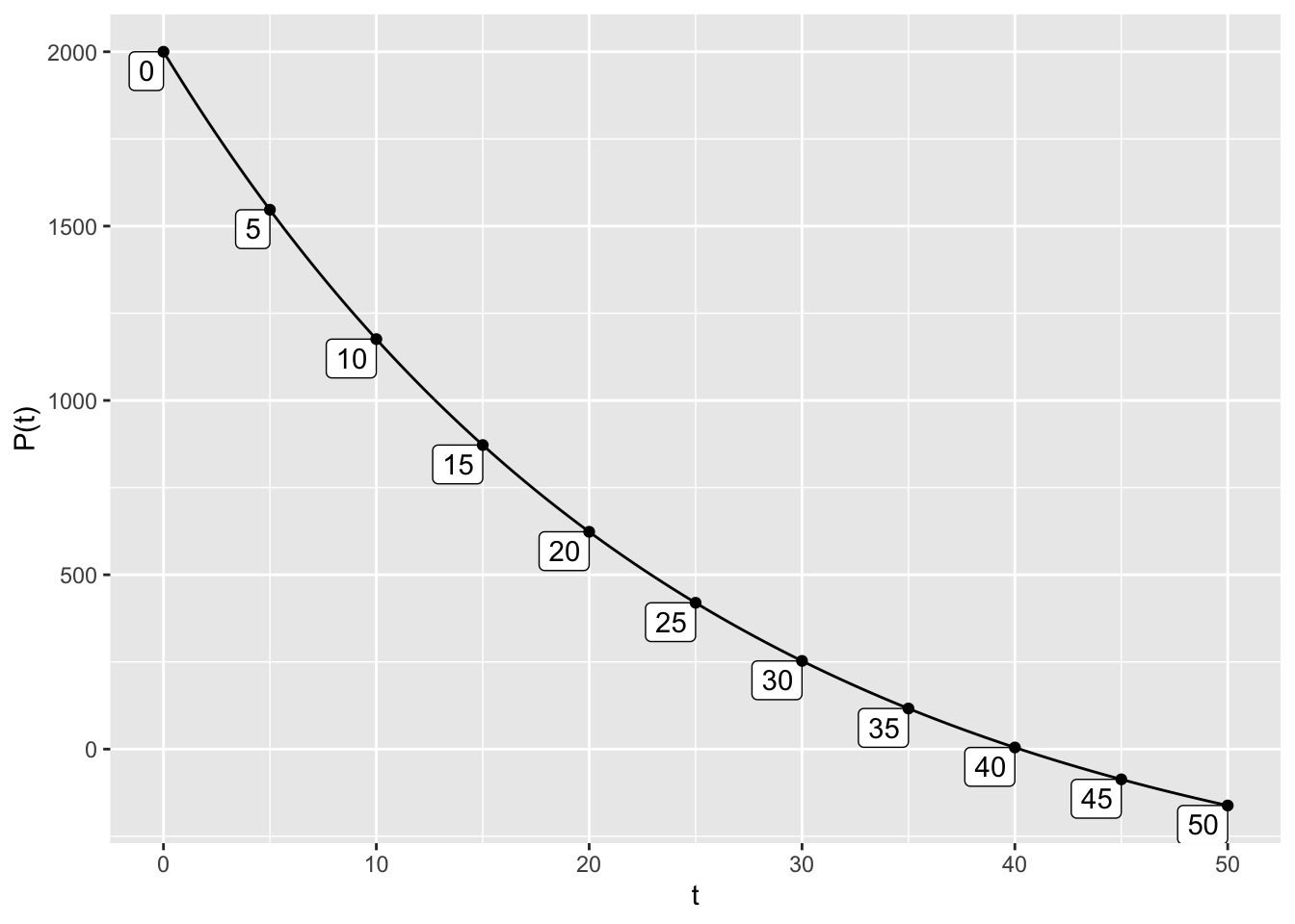

It takes about 40 days to clean up the pollutant. That is, \(P(40)=0\).

Slope Fields for Population Models

Exponential growth with harvesting.

vectorfield_plot(t ~ 1,
P ~  0.2 * P -  40,
domain(t=0:10, P=0:300))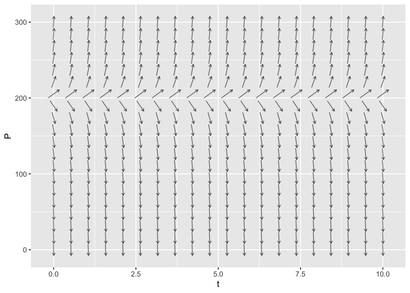

If \(P(0) > 200\) then the population increases without bound
If \(P(0) = 200\) then the population remains at this equilibrium value. This is an unstable equilibrium.
If \(P(0) < 200\) then the population decreases to zero.

Constrained growth

vectorfield_plot(t ~ 1,
P ~  0.05  * P *  (1 - 0.002 * P),
domain(t=0:50, P=0:600))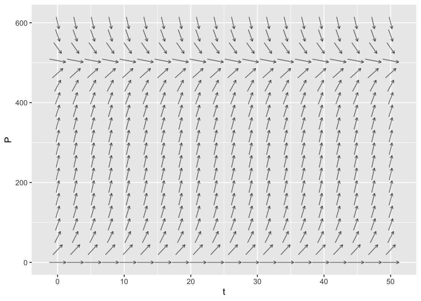

If \(P(0) = 0\) then the population remains at 0. This is an unstable equilibrium.
If \(0 < P(0) < 500\) then the population increases to the carrying capacity 500.
If \(P(0) = 500\) then the population remains at this equilibrium value. This is a stable equilibrium, and it is the carrying capacity.
If \(P(0) > 500\) then the population decreases down to the carrying capacity 500.

Constrained growth with constant harvesting

vectorfield_plot(t ~ 1,
P ~  0.05  * P *  (1 - 0.002 * P) - 4,
domain(t=0:50, P=0:600))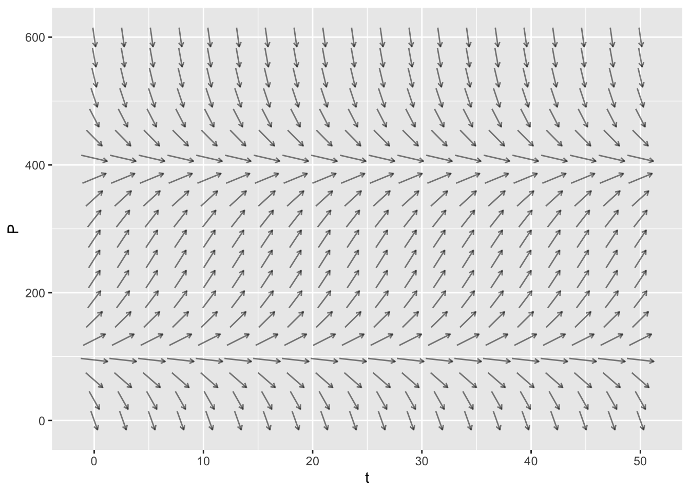

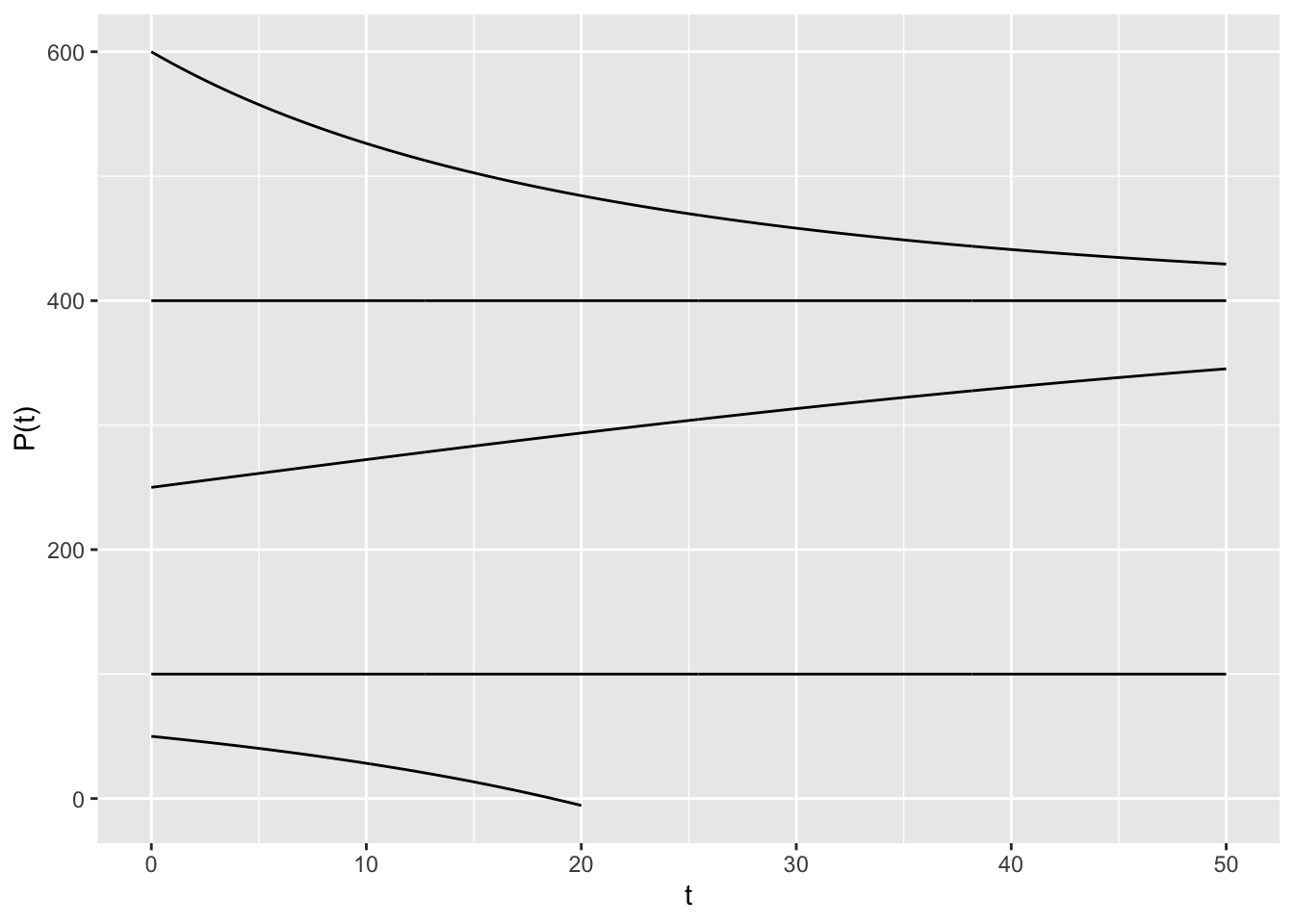
Let’s set \(\frac{dP}{dt}=0\) and solve to find the equilibrium points. We have \[\begin{align} -0.0001 P^2 + 0.05 P - 4 &= 0 \\ P^2 - 500 P + 40000 &= 0 \\ (P-100)(P-400) &= 0 \end{align}\]

If \(P(0) < 100\) then the population decreases to 0 at 0.
If \(P(0) = 100\) then the population remains at 100. This is an unstable equilibrium.
If \(100 < P(0) < 400\) then the population increases to 400.
If \(P(0) = 400\) then the population remains at this equilibrium value. This is a stable equilibrium.
If \(P(0) > 400\) then the population decreases down to 400.

Trajectories for Population Models

Exponential growth with harvesting. \[ \frac{dP}{dt} = 0.2 P - 40 \] for \(0 \leq P \leq 300\) and \(0 \leq t \leq 100\).

dyn = makeODE( dP ~  0.2 * P -  40 )
soln1 = integrateODE(dyn, domain(t=0:10), P=300)
soln2 = integrateODE(dyn, domain(t=0:10), P=200)
soln3 = integrateODE(dyn, domain(t=0:4), P=100)
traj_plot(P(t) ~ t, soln1,  nt=0) %>%
  traj_plot(P(t) ~ t, soln2,  nt=0) %>%
  traj_plot(P(t) ~ t, soln3,  nt=0)

Constrained growth \[ \frac{dP}{dt} = 0.05 P (1 - 0.002 P) \] for \(0 \leq P \leq 600\) and \(0 \leq t \leq 50\).

dyn = makeODE( dP ~  0.05 * P * (1 - 0.002 * P)  )
soln1 = integrateODE(dyn, domain(t=0:50), P=50)
soln2 = integrateODE(dyn, domain(t=0:50), P=100)
soln3 = integrateODE(dyn, domain(t=0:50), P=300)
soln4 = integrateODE(dyn, domain(t=0:50), P=500)
soln5 = integrateODE(dyn, domain(t=0:50), P=600)
traj_plot(P(t) ~ t, soln1,  nt=0) %>%
  traj_plot(P(t) ~ t, soln2,  nt=0) %>%
  traj_plot(P(t) ~ t, soln3,  nt=0) %>%
  traj_plot(P(t) ~ t, soln4,  nt=0) %>%
  traj_plot(P(t) ~ t, soln5,  nt=0)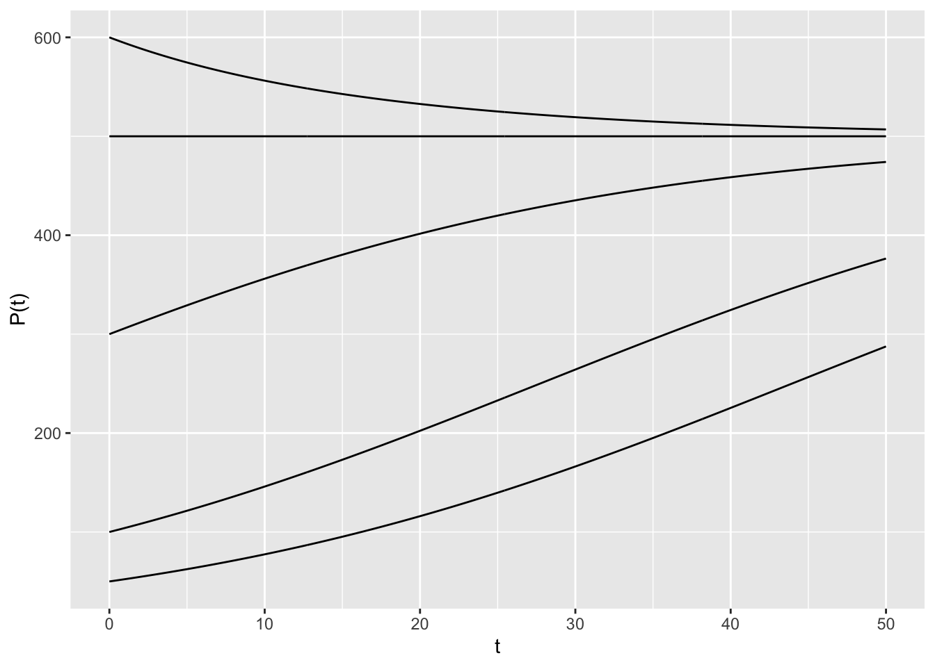

Constrained growth with constant harvesting \[ \frac{dP}{dt} = 0.05 P (1 - 0.002 P) - 4 \] for \(0 \leq P \leq 600\) and \(0 \leq t \leq 50\).

dyn = makeODE( dP ~  0.05 * P * (1 - 0.002 * P) -4  )
soln1 = integrateODE(dyn, domain(t=0:20), P=50)
soln2 = integrateODE(dyn, domain(t=0:50), P=100)
soln3 = integrateODE(dyn, domain(t=0:50), P=250)
soln4 = integrateODE(dyn, domain(t=0:50), P=400)
soln5 = integrateODE(dyn, domain(t=0:50), P=600)
traj_plot(P(t) ~ t, soln1,  nt=0) %>%
  traj_plot(P(t) ~ t, soln2,  nt=0) %>%
  traj_plot(P(t) ~ t, soln3,  nt=0) %>%
  traj_plot(P(t) ~ t, soln4,  nt=0) %>%
  traj_plot(P(t) ~ t, soln5,  nt=0)