7.C Euler’s Method
suppressPackageStartupMessages(library(mosaic))Introduction
Euler’s Method finds an approximate solution to a differential equation. Here is how it works. You are given
- The differential equation for \(\frac{dx}{dt}\).
- The initial point \((t_0,x_0)\).
- The step size \(\triangle t\).
- Either the number \(n\) of iterations, or the desired end time \(T\).
We want to find an approximation of the (unknown) function \(x(t)\).
We repeatedly use Local Linear Approximation to estimate the value of \(x(t)\) and times \(t_1=t_0+\triangle t\) and \(t_2=t_0+2\triangle t\) and \(t_3=t_0+3\triangle t\) and so on. Let’s call these estimates \(x_1, x_2, x_3\) and so on.
We estimate as follows: \[ \begin{array}{rcccl} x_1 &=& x_0 + x'(t_0) \cdot \triangle t \\ x_2 &=& x_1 + x'(t_1) \cdot \triangle t &=& x_1 + x'(t_0+\triangle t) \cdot \triangle t \\ x_3 &=& x_2 + x'(t_2) \cdot \triangle t &=& x_2 + x'(t_0+2 \triangle t) \cdot \triangle t \\ \end{array} \] We repeat \(n\) times. If we were given the ending time \(T\), then \(n= (T-t_0)/\triangle t\).
If you only want to calculate a few steps, then you can do this manually. But in general, we use RStudio to do the hard work.
Euler’s Method in RStudio
Here is code that uses Euler’s Method to find an approximate solution for the following problem:
- Differential equation \(\displaystyle{\frac{dx}{dt} = 3x - x^2}\)
- Initial point \(t_0=2\) and \(x_0= 5\)
- End time \(T=9\)
- Step size \(\triangle t = 0.01\)
# derivative, initial conditions and setup
dxdt = makeFun(3*x - x^2 ~ x)
tstart = 2
xstart = 5
tend = 9
dt = 0.01
num = (tend - tstart)/dt
# Euler's Method code
t = tstart
x = xstart
tlist = t
xlist = x
for (i in 1:num) {
  x = x + dt * dxdt(x)
  t = t + dt
  tlist = c(tlist, t)
  xlist = c(xlist, x)
}
# print the ending point
c(tail(tlist,1),  tail(xlist,1))
# plot the approximate function
gf_point(xlist ~ tlist) + xlab("t") + ylab("x(t)")
Activities
Euler’s Method for Two Steps
For each of the following problems, perform TWO steps of Euler’s Method for the given differential equation $, initial conditions and step size \(\triangle t\).
- Differential equation \(\displaystyle{\frac{dx}{dt} = x^2}\), initial conditions \(t_0=1\) and \(x_0= 3\) and step size \(\triangle t=1\).
- Differential equation \(\displaystyle{\frac{dx}{dt} = t^2}\), initial conditions \(t_0=1\) and \(x_0= 3\) and step size \(\triangle t=0.5\).
- Differential equation \(\displaystyle{\frac{dx}{dt} = t+x}\), initial conditions \(t_0=1\) and \(x_0= 3\) and step size \(\triangle t=0.25\).
Calculating an Euler Approximation
Use Euler’s Method to approximate the value \(x(4)\) where \(x(t)\) satisfies the differential equation \[ \frac{dx}{dt}=2x -6, \quad \mbox{where} \quad x(0)=4 \] by using times \(t_0=0\), \(t_1=0.5\), \(t_2=1.0\) and \(t_3 = 1.5\). Here is a table to get you started. \[ \begin{array}{c|c|c|c|c} n & t_n & x_n & x'(t_n) & x_{n} + x'(t_{n}) (t_{n+1} - t_{n}) \\ &&& = 2x_n - 6 & = x_{n} + x'(t_{n}) \cdot 0.5 \\ \hline 0 & 0 & 4 & 2 & \\ 1 & 0.5 & & \\ 2 & 1.0 & & \\ 3 & 1.5 & & \\ 4 & 2.0 & & \\ \end{array} \]
Estimating Drug Metabolization
Vancomycin is an antibiotic administered at a rate of 85 milligrams per hour and is metabolized at an hourly rate equal to 0.1 times the amount of drug in the body
- Write a differential equation relating \(\frac{dQ}{dt}\) and \(Q\), where \(Q\) is the quantity of the drug in the body.
- Modify the Euler’s Method code at the top of the page to plot a solution to your differential equation
- Start with initial condition \(Q(0)=0\).
- Use
dt=0.1 - Run the approximation for 1000 steps
- What happens to the amount of the drug in the body in the long run?
Medical doctors use this sort of calculation to maintain an effective dosage.
Euler’s Method with Different Step Sizes
We will use various step sizes in Euler’s method to estimate the value \(P(50)\) for the constrained growth problem \[ \frac{dP}{dt} = 0.04 P \left( 1 - \frac{P}{800} \right) \quad \mbox{and} \quad P(0)=100. \]
- Adapt the template Euler’s Method code at the top of this page to estimate \(P(50)\) when
- \(\triangle t = 10\)
- \(\triangle t = 1\)
- \(\triangle t = 0.1\)
- \(\triangle t = 0.01\)
- We know that the solution to this differential equation is a logistic function \(\displaystyle{P(t) = \frac{K}{1+Ce^{-rt}}}\). Find the values for \(r,C,K\). Then calculate the actual value of \(P(50)\) and compare this value our estimates. How did we do in each case?
Solutions
Euler’s Method for Two Steps
- We have \(\displaystyle{\frac{dx}{dt} = x^2}\), initial conditions \(t_0=1\) and \(x_0= 3\) and step size \(\triangle t=1\).
\[\begin{align} x_0 &=3 \\ x_1 &= 3 + 3^2 \cdot 1 = 12 \\ x_2 &= 12 + 12^2 \cdot 1 = 12+ 144 = 156 \end{align}\]
- We have \(\displaystyle{\frac{dx}{dt} = t^2}\), initial conditions \(t_0=1\) and \(x_0= 3\) and step size \(\triangle t=0.5\).
\[\begin{align} x_0 &=3 \\ x_1 &= 3 + 1^2 \cdot 0.5 = 3.5 \\ x_2 &= 3.5 + (3.5)^2 \cdot 0.5 = 3.5 + 6.125 = 9.625 \end{align}\]
- We have \(\displaystyle{\frac{dx}{dt} = t+x}\), initial conditions \(t_0=1\) and \(x_0= 3\) and step size \(\triangle t=0.25\).
\[\begin{align} x_0 &=3 \\ x_1 &= 3 + (1+3) \cdot 0.25 = 3+ 1 = 4 \\ x_2 &= 4 + (0.25+4) \cdot 0.25 = 4 + 1.0625 = 5.0625 \end{align}\]
Calculating an Euler Approximation
We run Euler’s Method for 4 steps. \[ \begin{array}{c|c|c|c|c} n & t_n & x_n & x'(t_n) & x_{n} + x'(t_{n}) (t_{n+1} - t_{n}) \\ &&& = 2x_n - 6 & = x_{n} + x'(t_{n}) \cdot 0.5 \\ \hline 0 & 0 & 4 & 2 & 4 + 2 \cdot 0.5 = 4+1 = 5 \\ 1 & 0.5 & 5 & 4 & 5 + 4 \cdot 0.5 = 5+2=7 \\ 2 & 1.0 & 7 & 8 & 7 + 8 \cdot 0.5 = 7+4=11 \\ 3 & 1.5 & 11 & 18 & 11 + 18 \cdot 0.5 = 11 + 9 =20 \\ 4 & 2.0 & 20 & \\ \end{array} \]
Estimating Drug Metabolization
- Our differential equation is \[ \frac{dQ}{dt} = -0.1 Q + 85 \]
- We run the Euler’s Method code with \(Q(0)=0\) and
dt=0.1for 1000 steps
# derivative, initial conditions and setup
dxdt = makeFun(-0.1*x + 85 ~ x)
tstart = 0
xstart = 0
dt = 0.1
num = 1000
# Euler's Method code
t = tstart
x = xstart
tlist = t
xlist = x
for (i in 1:num) {
  x = x + dt * dxdt(x)
  t = t + dt
  tlist = c(tlist, t)
  xlist = c(xlist, x)
}
# print the ending point
c(tail(tlist,1),  tail(xlist,1))
## [1] 100.0000 849.9633# plot the approximate function
gf_point(xlist ~ tlist) + xlab("time") + ylab("Q(t)")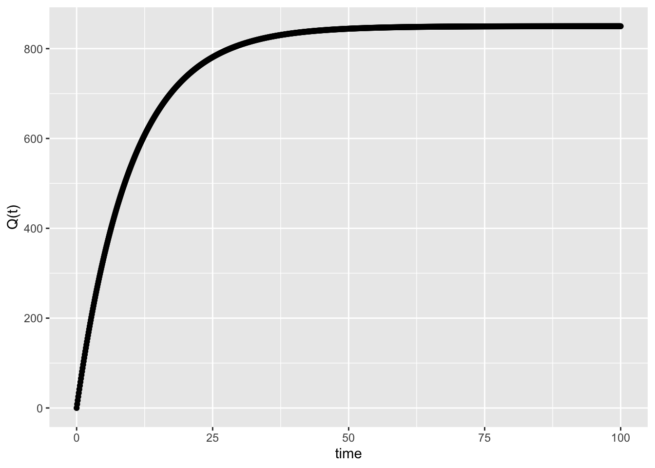
- The amount of the drug converges to 850.
Euler’s Method with Different Step Sizes
We will use various step sizes in Euler’s method to estimate the value \(P(50)\) for the constrained growth problem \[ \frac{dP}{dt} = 0.04 P \left( 1 - \frac{P}{800} \right) \quad \mbox{and} \quad P(0)=100. \]
- We use Euler’s Method code to estimate \(P(50)\) when
- \(\triangle t = 10\)
# derivative, initial conditions and setup
dxdt = makeFun(0.04*x*(1-x/800) ~ x)
tstart = 0
xstart = 100
tend = 50
dt = 10
num = (tend - tstart)/dt
# Euler's Method code
t = tstart
x = xstart
tlist = t
xlist = x
for (i in 1:num) {
  x = x + dt * dxdt(x)
  t = t + dt
  tlist = c(tlist, t)
  xlist = c(xlist, x)
}
# print the ending point
c(tail(tlist,1),  tail(xlist,1))
## [1] 50.000 377.373# plot the approximate function
gf_point(xlist ~ tlist) + xlab("time") + ylab("P(t)")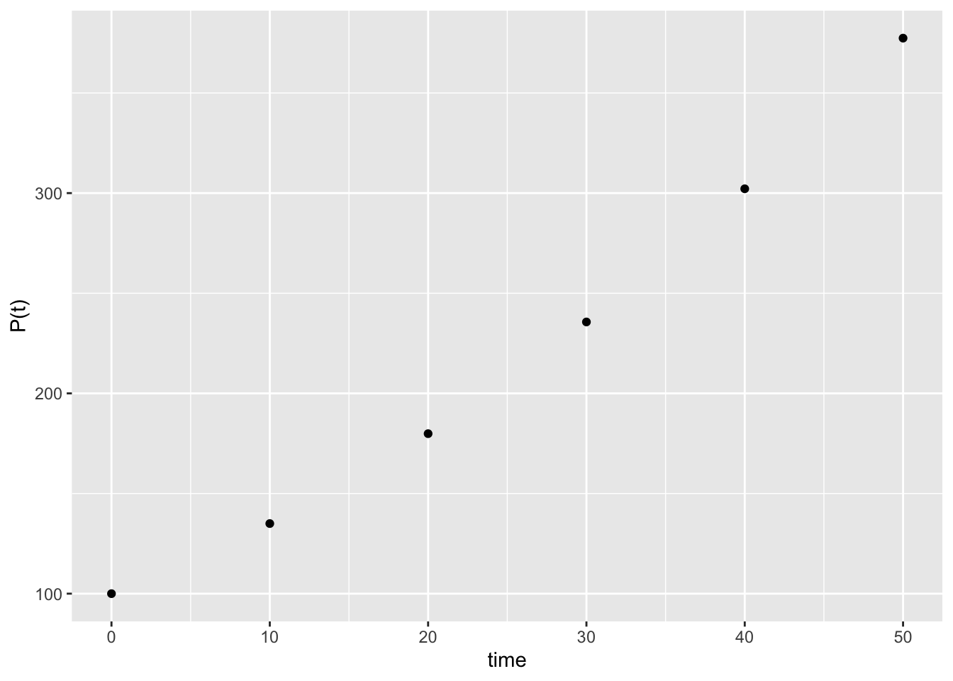
- \(\triangle t = 1\)
# derivative, initial conditions and setup
dxdt = makeFun(0.04*x*(1-x/800) ~ x)
tstart = 0
xstart = 100
tend = 50
dt = 1
num = (tend - tstart)/dt
# Euler's Method code
t = tstart
x = xstart
tlist = t
xlist = x
for (i in 1:num) {
  x = x + dt * dxdt(x)
  t = t + dt
  tlist = c(tlist, t)
  xlist = c(xlist, x)
}
# print the ending point
c(tail(tlist,1),  tail(xlist,1))
## [1] 50.0000 407.5033# plot the approximate function
gf_point(xlist ~ tlist) + xlab("time") + ylab("P(t)")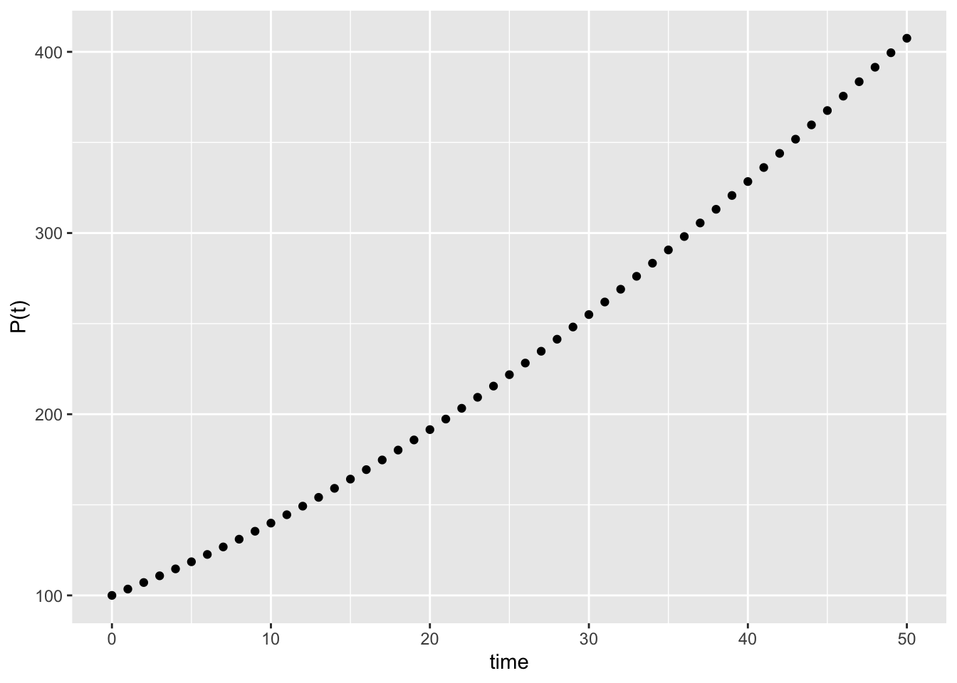
- \(\triangle t = 0.1\)
# derivative, initial conditions and setup
dxdt = makeFun(0.04*x*(1-x/800) ~ x)
tstart = 0
xstart = 100
tend = 50
dt = 0.1
num = (tend - tstart)/dt
# Euler's Method code
t = tstart
x = xstart
tlist = t
xlist = x
for (i in 1:num) {
  x = x + dt * dxdt(x)
  t = t + dt
  tlist = c(tlist, t)
  xlist = c(xlist, x)
}
# print the ending point
c(tail(tlist,1),  tail(xlist,1))
## [1] 50.0000 410.4851# plot the approximate function
gf_point(xlist ~ tlist) + xlab("time") + ylab("P(t)")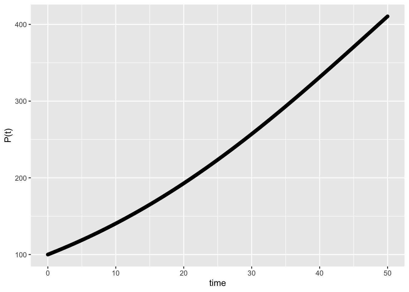
- \(\triangle t = 0.01\)
# derivative, initial conditions and setup
dxdt = makeFun(0.04*x*(1-x/800) ~ x)
tstart = 0
xstart = 100
tend = 50
dt = 0.01
num = (tend - tstart)/dt
# Euler's Method code
t = tstart
x = xstart
tlist = t
xlist = x
for (i in 1:num) {
  x = x + dt * dxdt(x)
  t = t + dt
  tlist = c(tlist, t)
  xlist = c(xlist, x)
}
# print the ending point
c(tail(tlist,1),  tail(xlist,1))
## [1] 50.0000 410.7823# plot the approximate function
gf_point(xlist ~ tlist) + xlab("time") + ylab("P(t)")
- We have \[ P(t) = \frac{800}{1+Ce^{-0.04t}} \qquad \mbox{and} \qquad P(0)=100 \] so \(C=7\) and our function is \[ P(t) = \frac{800}{1+7e^{-0.04t}}. \] Evaluting at \(t=50\) gives \[ P(50)=410.8153. \] The estimates when \(\triangle t=0.1\) and \(\triangle t=0.01\) are very good!