1.G Multivariable Functions
Goals
- Identify and explain independent and dependent variables in multivariable functions
- Interpret functions represented as tables and equations
- Interpret contour diagrams and make function value estimates
- Interpret cross sections and connect them with contour diagrams
- Use RStudio to create a contour plot and a surface plot of a function \(z=f(x,y)\).
Activities
Plotting in RStudio
Create these plots using RStudio.
You will need to import the mosaic package and the mosaicCalc package. Cut and paste this code chunk into your RMD file and run it. This will load in the slice_plot, interactive_plot and contour_plot commands.
```{r setup, include=FALSE, warning=FALSE}
knitr::opts_chunk$set(echo = TRUE)
suppressPackageStartupMessages(library(mosaic))
suppressPackageStartupMessages(library(mosaicCalc))
```- Windchill Function
\[ W(T,V) = 35.74+0.6215 \, T-35.75 \, V^{0.16}+0.4275 \, T \, V^{0.16} \]
Surface plot
W = makeFun(35.74+0.6215*T-35.75*V^(0.16)+0.4275*T*V^(0.16) ~ T & V)

interactive_plot(W(T,V) ~ T & V,
        domain(T=-40:40,V=5:60))
Contour Plot
contour_plot(W(T,V) ~ T & V,
        domain(T=-40:40,V=5:60),
        skip=0)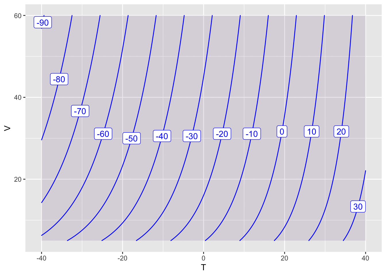
- Another Function
\[ f(x,y) = \frac{\sin(x^2+y^2)}{0.1+x^2+y^2}+ \frac{1}{2}(x^2+4y^2)e^{1-x^2-y^2} \] Surface Plot
f = makeFun(sin(x^2+y^2)/(0.1+x^2+y^2)+(x^2+4*y^2)*exp(1-x^2-y^2)/2~ x & y)

interactive_plot(f(x,y) ~ x & y,
        domain(x=-2:2, y=-2:2))
Contour Plot
contour_plot(f(x,y) ~ x & y,
        domain(x=-2:2, y=-2:2),
        skip=0)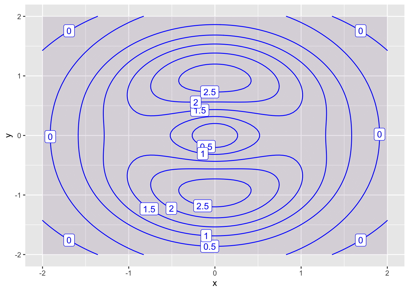
Cross Sections
For each of the the two functions in the previous problem:
- Sketch two or three horizontal cross sections
- Sketch two or three vertical cross sections
- Then use RStudio to create these cross sections and compare to your sketches. How well did you do?
Plotting in RStudio
Here is some sample RStudio code that defines a function P(x,y) = x^2 - 4x y^3 and then creates two contour plots. The first plot uses the default contours. The second plot uses the given list of contours.
P = makeFun(x^2 - 4*x*y^3 ~ x&y)

contour_plot(P(x,y) ~ x&y,
             domain(x=-5:5, y=-5:5),
             skip=0)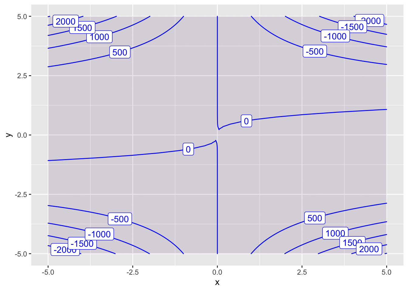
contour_plot(P(x,y) ~ x&y,
             domain(x=-5:5, y=-5:5),
             contours_at = seq(-2000,2000,250),
             skip=0)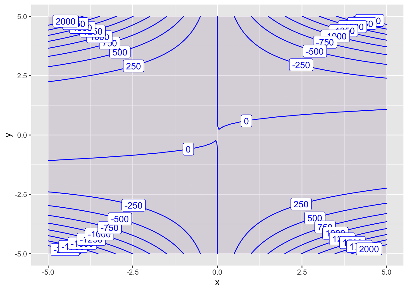
Using RStudio,
- Use
makeFunto create each of these functions. - Then use
contour_plotto create a contour plot.
Try out different horizontal and vertical domains that are centered around the origin. Change the level curves.
- \(f(x,y) = \sin(\sqrt{x^2+y^2})\)
- \(g(x,y) = 100 x^2 y^2 e^{-x^2-y^2}\)
- \(h(x,y) = \sin^2x + \frac{1}{4}y^2\)
Solutions
Cross Sections
- Here are some cross sections for the windchill function \[W(T,V) = 35.74+0.6215 \, T-35.75 \, V^{0.16}+0.4275 \, T \, V^{0.16}\]
W = makeFun(35.74+0.6215*T-35.75*V^(0.16)+0.4275*T*V^(0.16)~T & V)

slice_plot(W(T,20) ~ T,
        domain(T=-40:40)) + labs(title="Windchill for V=20") + ylab("W")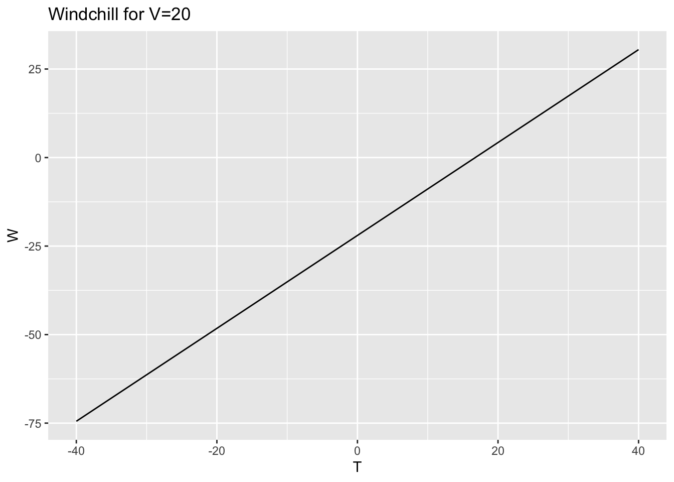
slice_plot(W(T,40) ~ T,
        domain(T=-40:40)) + labs(title="Windchill for W=20") + ylab("W")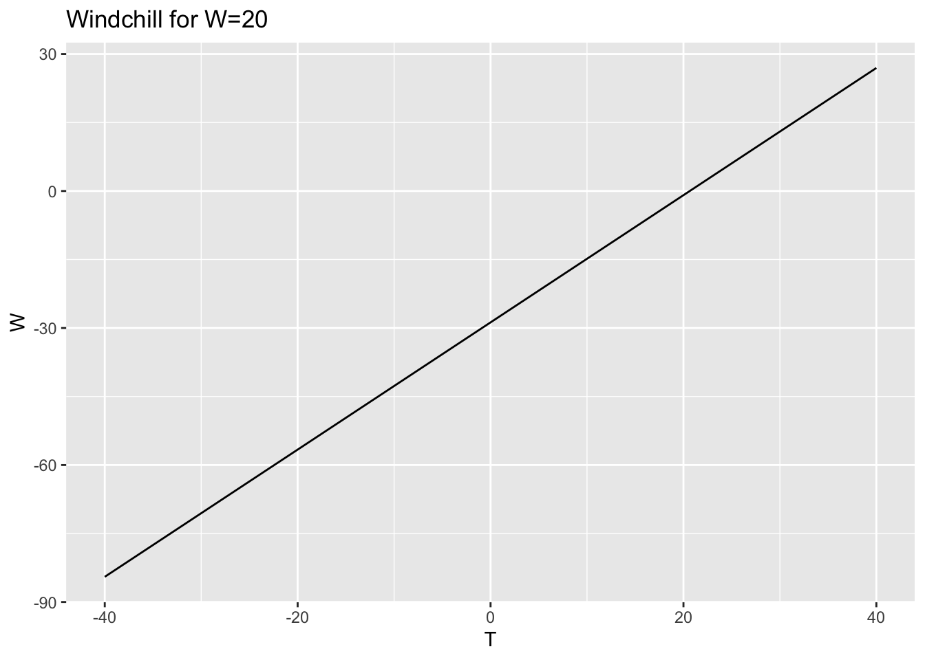
slice_plot(W(-20,V) ~ V,
        domain(V=0:60)) + labs(title="Windchill for T=-20") + ylab("W")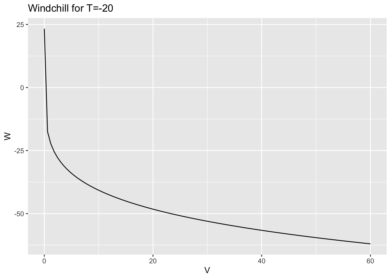
slice_plot(W(10,V) ~ V,
        domain(V=0:60)) + labs(title="Windchill for T=10") + ylab("W")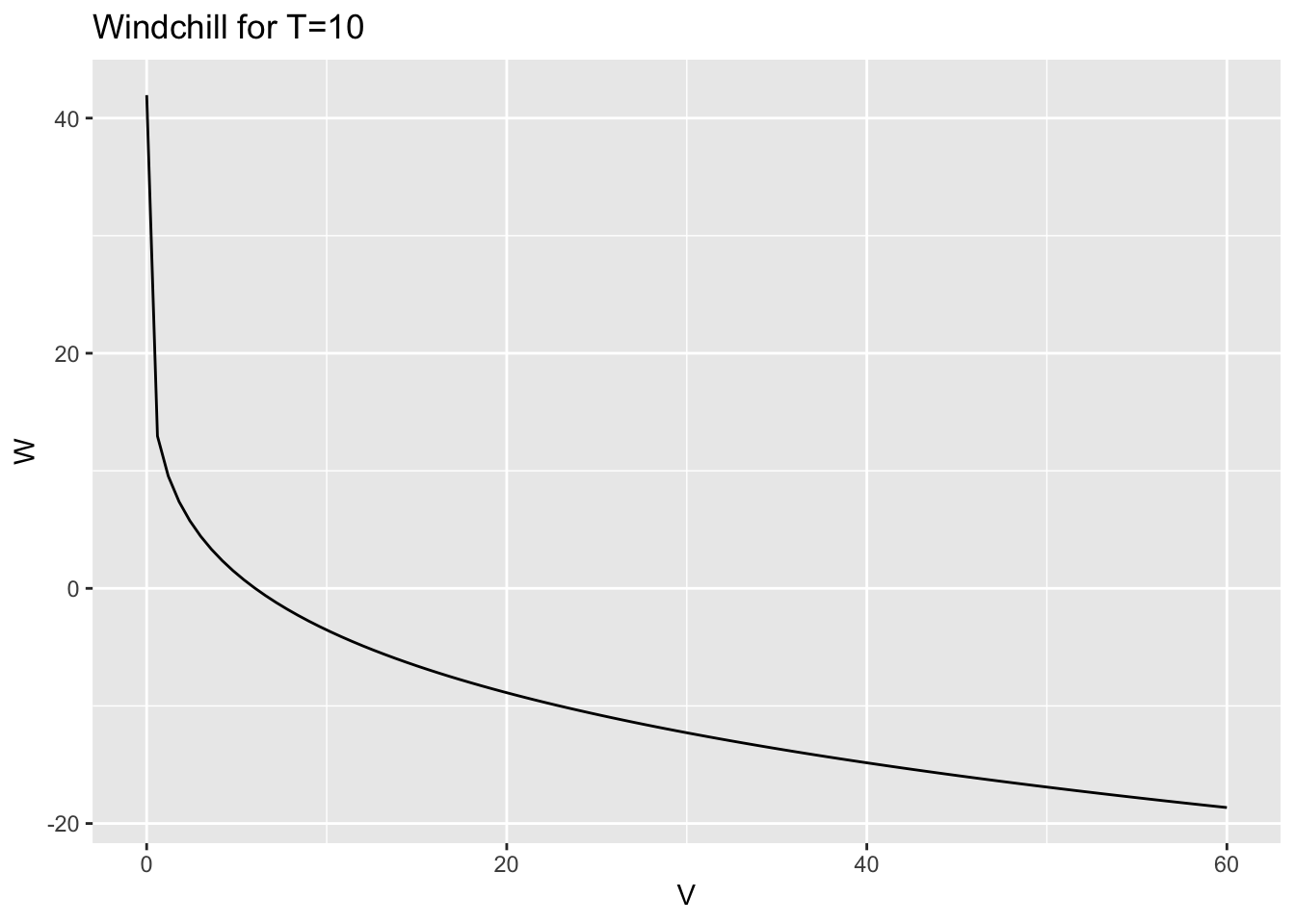
- Here are some cross sections for the second function. \[ f(x,y) = \frac{\sin(x^2+y^2)}{0.1+x^2+y^2}+ \frac{1}{2}(x^2+4y^2)e^{1-x^2-y^2} \]
f = makeFun(sin(x^2 + y^2)/(0.1 + x^2 + y^2) + (x^2 + 4*y^2) * exp(1 - x^ 2- y^2)/2 ~ x & y)slice_plot(f(x,-1.5) ~ x, domain(x=-1:1)) + ylab("f(x,-1.5)")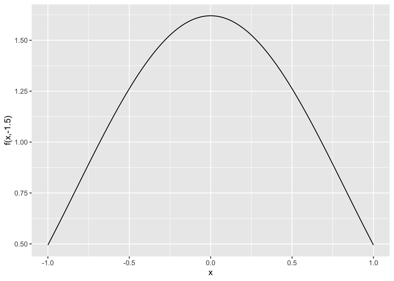
slice_plot(f(x,0) ~ x, domain(x=-1:1)) + ylab("f(x,0)")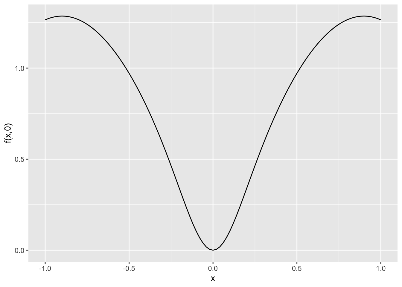
slice_plot(f(x,1.5) ~ x, domain(x=-1:1)) + ylab("f(x,1.5)")
slice_plot(f(-1.5,y) ~ y, domain(y=-1:1)) + ylab("f(-1.5,y)")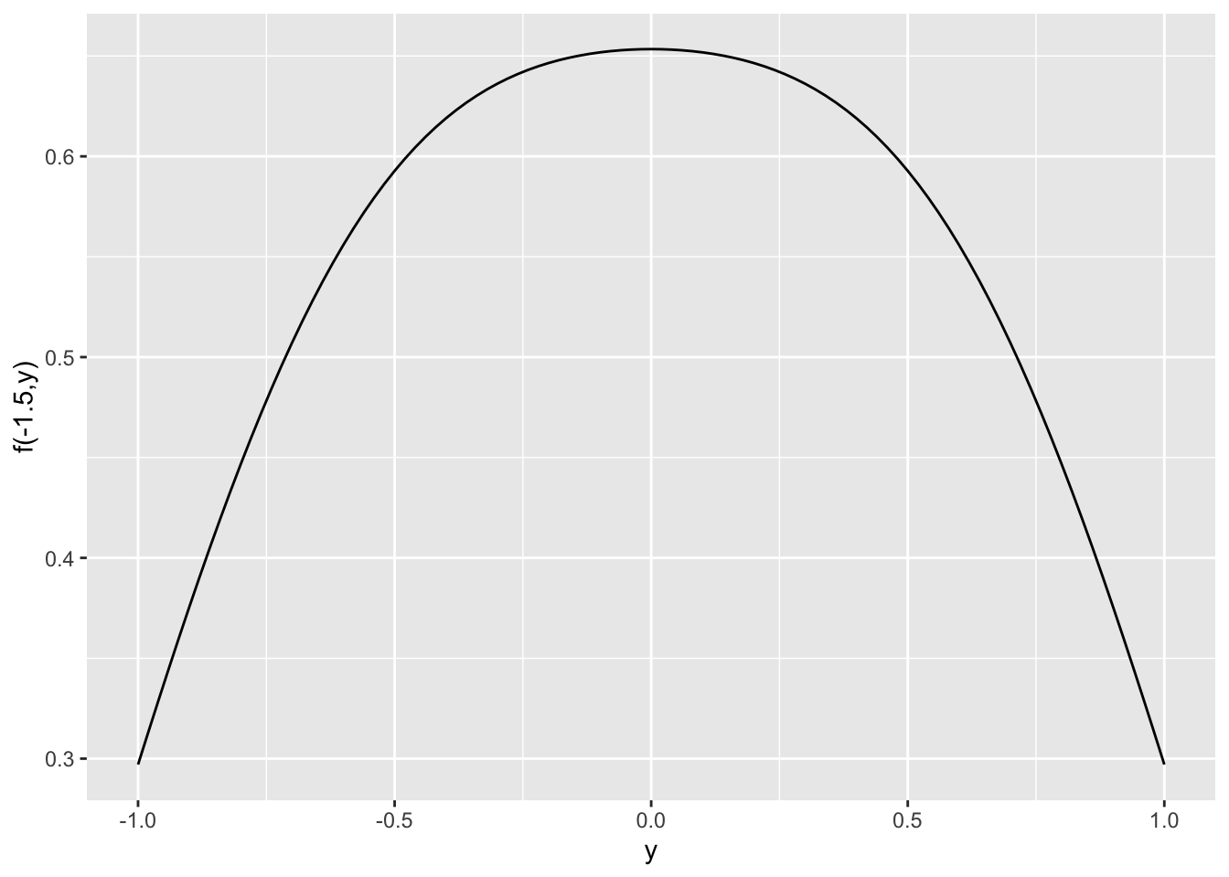
slice_plot(f(0,y) ~ y, domain(y=-1:1)) + ylab("f(0,y)")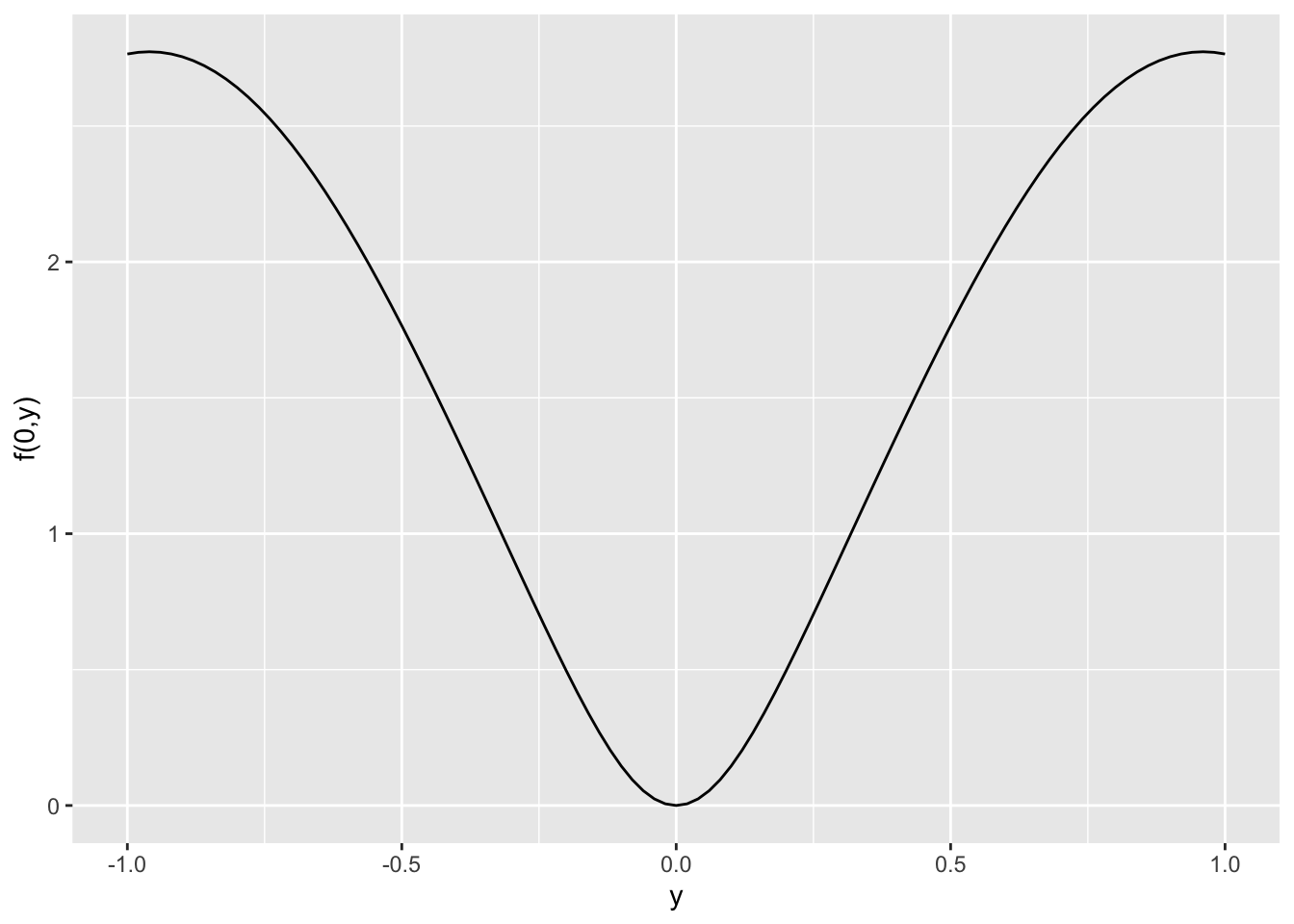
slice_plot(f(1.5,y) ~ y, domain(y=-1:1)) + ylab("f(1.5,y)")
Plotting in RStudio
- \(f(x,y) = \sin(\sqrt{x^2+y^2})\)
f = makeFun(sin( sqrt((x^2+y^2))) ~ x&y)

contour_plot(f(x,y) ~ x & y,
        domain(x=-3:3, y=-3:3),
        skip=0)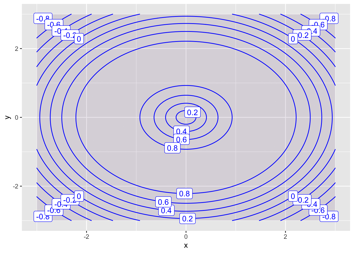
- \(g(x,y) = x^2 y^2 e^{-x^2-y^2}\)
g = makeFun(100 * x^2 *  y^2 * exp(-x^2-y^2) ~ x&y)

contour_plot(g(x,y) ~ x & y,
        domain(x=-2:2,y=-2:2),
        contours_at = seq(0,14,2),
        skip=0)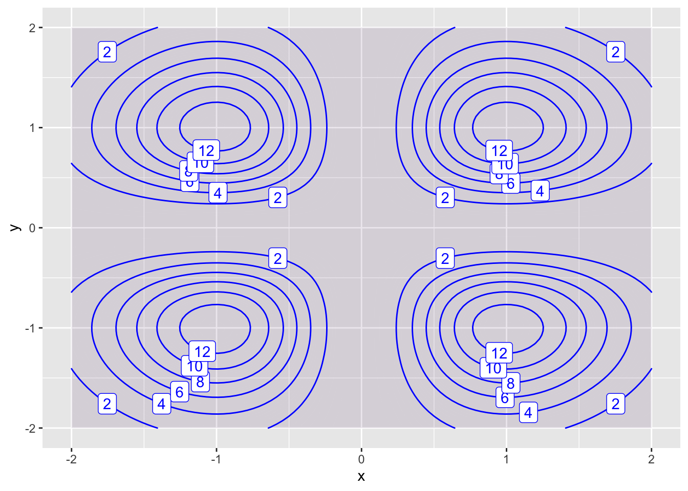
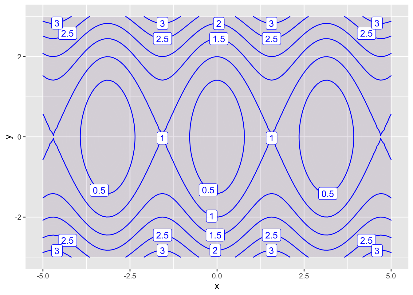
- \(h(x,y) = \sin^2x + \frac{1}{4}y^2\)
g = makeFun((sin(x))^2 + y^2/4 ~ x&y)

contour_plot(g(x,y) ~ x & y,
        domain(x=-5:5, y=-3:3),
        contours_at=seq(0,4,0.5),
        skip=0)