Vector 23 Voting Patterns in the US Senate
In 2014, the Pew Research Center published a report about the increasing polarization of US politics. They wrote:
Republicans and Democrats are more divided along ideological lines – and partisan antipathy is deeper and more extensive – than at any point in the last two decades. These trends manifest themselves in myriad ways, both in politics and in everyday life.
Is this really true, or is this just hype? Let’s see what linear algebra can tell us about the evolution of voting patterns in the US Senate from 1964 to 2012.
23.1 The Data
We will analyze datasets corresponding to US Senate votes during a 2-year Congressional Session. Our data sets are 12 years apart, and were chosen to coincide with US election years.
| Session | Years | US Election | # Floor Votes |
|---|---|---|---|
| 84 | 1963-1965 | Lyndon Johnson vs Richard Nixon | 534 |
| 94 | 1975-1977 | Jimmy Carter vs Gerald Ford | 1311 |
| 100 | 1987-1989 | George H. W. Bush vs Michael Dukakis | 799 |
| 106 | 1999-2001 | George W. Bush vs Al Gore | 672 |
| 112 | 2011-2013 | Barack Obama vs John McCain | 486 |
Here is a list our our data files, which we will load from Github. The original data can be found at voteview.com. There are two files for each year.
- A csv file containing a matrix whose \((i,j)\) entry counts the number of times Senator \(i\) and Senator \(j\) cast the same vote on an issue. There are actually nine different possibilities, including Yea, Nay, Present, Abstention and “Not a member of the chamber when the vote was taken.”
- A csv file containing senator information: name, state and party affiliation.
senate.1964.files = c('https://raw.github.com/mathbeveridge/math236_f20/main/data/Senate088matrix.csv', 'https://raw.github.com/mathbeveridge/math236_f20//main/data/Senate088senators.csv')

senate.1976.files = c('https://raw.github.com/mathbeveridge/math236_f20/main/data/Senate094matrix.csv', 'https://raw.github.com/mathbeveridge/math236_f20//main/data/Senate094senators.csv')

senate.1988.files = c('https://raw.github.com/mathbeveridge/math236_f20/main/data/Senate100matrix.csv', 'https://raw.github.com/mathbeveridge/math236_f20//main/data/Senate100senators.csv')

senate.2000.files = c('https://raw.github.com/mathbeveridge/math236_f20/main/data/Senate106matrix.csv', 'https://raw.github.com/mathbeveridge/math236_f20//main/data/Senate106senators.csv')

senate.2012.files = c('https://raw.github.com/mathbeveridge/math236_f20/main/data/Senate112matrix.csv', 'https://raw.github.com/mathbeveridge/math236_f20//main/data/Senate112senators.csv')
23.2 The 88th Congressional Session (1964)
Let’s load in our data.
# pick the data set that we want to look at
senate.files = senate.1964.files


# First we load in the information about the senators.
# We will use these names as our labels.
# We also set up the colors we will use for our data points.
senators <- read.csv(senate.files[2], header=FALSE)

sen.name = senators[,2]
sen.party = senators[,4]

sen.color=rep("goldenrod", length(senators))
sen.color[sen.party=='D']="cornflowerblue"
sen.color[sen.party=='R']="firebrick"


# Next we load in the square matrix that measures how often senators voted together.
# We add names for the columns and rows.
votes <- read.csv(senate.files[1], header=FALSE)
names(votes) <- sen.name
row.names(votes) <- sen.name


knitr::kable(
  head(votes), booktabs = TRUE,
  caption = 'Congressional Sessions of the US Senate'
)| AIKEN George David | ALLOTT Gordon Llewellyn | ANDERSON Clinton Presba | BARTLETT Edward Lewis (Bob) | BEALL James Glenn | BENNETT Wallace Foster | BIBLE Alan Harvey | BOGGS James Caleb | BREWSTER Daniel Baugh | BURDICK Quentin Northrup | BYRD Harry Flood | BYRD Robert Carlyle | CANNON Howard Walter | CARLSON Frank | CASE Clifford Philip | CHURCH Frank Forrester | CLARK Joseph Sill | COOPER John Sherman | COTTON Norris H. | CURTIS Carl Thomas | DIRKSEN Everett McKinley | DODD Thomas Joseph | DOUGLAS Paul Howard | EASTLAND James Oliver | ELLENDER Allen Joseph | ENGLE Clair | ERVIN Samuel James Jr. | FONG Hiram Leong | FULBRIGHT James William | GOLDWATER Barry Morris | GORE Albert Arnold | GRUENING Ernest Henry | HART Philip Aloysius | HARTKE Rupert Vance | HAYDEN Carl Trumbull | HICKENLOOPER Bourke Blakemore | HILL Joseph Lister | HOLLAND Spessard Lindsey | HRUSKA Roman Lee | HUMPHREY Hubert Horatio Jr. | INOUYE Daniel Ken | JACKSON Henry Martin (Scoop) | JAVITS Jacob Koppel | JOHNSTON Olin DeWitt Talmadge | JORDAN Benjamin Everett | KEATING Kenneth Barnard | KEFAUVER Carey Estes | KUCHEL Thomas Henry | LAUSCHE Frank John | LONG Edward Vaughn | LONG Russell Billiu | MAGNUSON Warren Grant | MANSFIELD Michael Joseph (Mike) | McCARTHY Eugene Joseph | McCLELLAN John Little | McGEE Gale William | McGOVERN George Stanley | McNAMARA Patrick Vincent | METCALF Lee Warren | MONRONEY Almer Stillwell Mike | MORSE Wayne Lyman | MORTON Thruston Ballard | MOSS Frank Edward (Ted) | MUNDT Karl Earl | MUSKIE Edmund Sixtus | NEUBERGER Maurine Brown | PASTORE John Orlando | PROUTY Winston Lewis | PROXMIRE William | RANDOLPH Jennings | RIBICOFF Abraham Alexander | ROBERTSON Absalom Willis | RUSSELL Richard Brevard Jr. | SALTONSTALL Leverett | SCOTT Hugh Doggett Jr. | SMATHERS George Armistead | SMITH Margaret Chase | SPARKMAN John Jackson | STENNIS John Cornelius | SYMINGTON William Stuart (Stuart) | TALMADGE Herman Eugene | WILLIAMS Harrison Arlington Jr. | WILLIAMS John James | YARBOROUGH Ralph Webster | YOUNG Milton Ruben | YOUNG Stephen Marvin | DOMINICK Peter Hoyt | BAYH Birch Evans | EDMONDSON James Howard | JORDAN Leonard Beck (Len) | KENNEDY Edward Moore (Ted) | McINTYRE Thomas James | MECHEM Edwin Leard | MILLER Jack Richard | NELSON Gaylord Anton | PEARSON James Blackwood | PELL Claiborne de Borda | SIMPSON Milward Lee | TOWER John Goodwin | THURMOND James Strom | WALTERS Herbert Sanford | SALINGER Pierre Emil George | |
|---|---|---|---|---|---|---|---|---|---|---|---|---|---|---|---|---|---|---|---|---|---|---|---|---|---|---|---|---|---|---|---|---|---|---|---|---|---|---|---|---|---|---|---|---|---|---|---|---|---|---|---|---|---|---|---|---|---|---|---|---|---|---|---|---|---|---|---|---|---|---|---|---|---|---|---|---|---|---|---|---|---|---|---|---|---|---|---|---|---|---|---|---|---|---|---|---|---|---|---|---|---|---|
| AIKEN George David | 0 | 321 | 252 | 302 | 336 | 287 | 282 | 384 | 286 | 297 | 155 | 246 | 245 | 318 | 366 | 294 | 254 | 316 | 259 | 248 | 302 | 301 | 322 | 172 | 175 | 58 | 201 | 377 | 183 | 128 | 215 | 248 | 292 | 259 | 185 | 308 | 198 | 218 | 243 | 310 | 326 | 302 | 339 | 183 | 199 | 379 | 33 | 394 | 287 | 275 | 155 | 262 | 258 | 278 | 201 | 288 | 298 | 285 | 289 | 301 | 265 | 266 | 280 | 306 | 316 | 256 | 320 | 425 | 334 | 292 | 318 | 173 | 181 | 326 | 321 | 160 | 416 | 217 | 187 | 292 | 190 | 305 | 296 | 219 | 290 | 296 | 286 | 287 | 227 | 323 | 221 | 331 | 215 | 328 | 316 | 297 | 306 | 248 | 187 | 182 | 124 | 26 |
| ALLOTT Gordon Llewellyn | 321 | 0 | 221 | 251 | 293 | 326 | 266 | 344 | 237 | 250 | 171 | 196 | 234 | 322 | 289 | 237 | 172 | 296 | 260 | 286 | 286 | 255 | 239 | 163 | 193 | 50 | 191 | 326 | 137 | 139 | 157 | 218 | 219 | 200 | 147 | 287 | 179 | 227 | 269 | 235 | 257 | 271 | 272 | 169 | 205 | 296 | 14 | 310 | 285 | 237 | 141 | 237 | 203 | 222 | 211 | 235 | 230 | 204 | 227 | 253 | 230 | 285 | 235 | 323 | 246 | 178 | 239 | 340 | 278 | 240 | 247 | 204 | 177 | 284 | 292 | 127 | 323 | 183 | 199 | 244 | 196 | 232 | 288 | 190 | 294 | 228 | 339 | 221 | 225 | 344 | 159 | 263 | 244 | 320 | 236 | 327 | 234 | 321 | 240 | 208 | 129 | 17 |
| ANDERSON Clinton Presba | 252 | 221 | 0 | 304 | 258 | 175 | 302 | 248 | 322 | 303 | 106 | 254 | 298 | 215 | 290 | 287 | 279 | 227 | 170 | 142 | 187 | 286 | 279 | 138 | 161 | 82 | 173 | 256 | 193 | 114 | 213 | 256 | 308 | 284 | 213 | 180 | 186 | 179 | 132 | 303 | 338 | 287 | 276 | 203 | 190 | 280 | 40 | 284 | 190 | 265 | 178 | 278 | 255 | 296 | 155 | 276 | 308 | 305 | 303 | 310 | 255 | 191 | 298 | 201 | 321 | 253 | 301 | 235 | 271 | 283 | 303 | 129 | 136 | 223 | 248 | 186 | 295 | 200 | 165 | 289 | 182 | 299 | 166 | 238 | 219 | 263 | 182 | 302 | 290 | 203 | 280 | 332 | 135 | 215 | 299 | 214 | 289 | 144 | 111 | 114 | 137 | 21 |
| BARTLETT Edward Lewis (Bob) | 302 | 251 | 304 | 0 | 288 | 201 | 363 | 291 | 349 | 386 | 133 | 318 | 323 | 258 | 335 | 359 | 335 | 264 | 182 | 162 | 213 | 351 | 355 | 150 | 187 | 83 | 196 | 313 | 237 | 75 | 264 | 340 | 370 | 328 | 252 | 216 | 245 | 221 | 154 | 395 | 419 | 349 | 332 | 263 | 230 | 332 | 48 | 317 | 205 | 328 | 209 | 335 | 325 | 361 | 196 | 362 | 377 | 375 | 374 | 389 | 328 | 208 | 334 | 230 | 401 | 327 | 377 | 284 | 336 | 349 | 379 | 162 | 175 | 249 | 286 | 215 | 334 | 250 | 185 | 333 | 206 | 378 | 193 | 285 | 256 | 326 | 200 | 348 | 291 | 220 | 292 | 400 | 141 | 233 | 379 | 215 | 377 | 159 | 110 | 144 | 150 | 37 |
| BEALL James Glenn | 336 | 293 | 258 | 288 | 0 | 274 | 290 | 357 | 279 | 290 | 170 | 227 | 249 | 307 | 330 | 250 | 243 | 278 | 268 | 249 | 254 | 315 | 306 | 152 | 156 | 57 | 191 | 355 | 168 | 149 | 194 | 256 | 286 | 270 | 174 | 271 | 183 | 194 | 255 | 280 | 310 | 292 | 327 | 201 | 207 | 367 | 24 | 352 | 248 | 264 | 158 | 256 | 223 | 260 | 188 | 262 | 276 | 266 | 258 | 275 | 275 | 255 | 247 | 295 | 284 | 241 | 292 | 349 | 326 | 286 | 310 | 175 | 182 | 287 | 347 | 145 | 368 | 179 | 170 | 307 | 198 | 295 | 278 | 216 | 267 | 293 | 292 | 266 | 236 | 318 | 219 | 315 | 238 | 304 | 295 | 306 | 289 | 249 | 225 | 189 | 124 | 32 |
| BENNETT Wallace Foster | 287 | 326 | 175 | 201 | 274 | 0 | 249 | 337 | 178 | 183 | 238 | 198 | 212 | 296 | 233 | 185 | 135 | 270 | 317 | 343 | 290 | 199 | 189 | 212 | 226 | 37 | 244 | 284 | 162 | 220 | 162 | 200 | 167 | 156 | 124 | 336 | 189 | 238 | 328 | 176 | 205 | 215 | 223 | 203 | 231 | 251 | 14 | 263 | 282 | 188 | 191 | 178 | 151 | 163 | 241 | 189 | 176 | 161 | 173 | 208 | 203 | 267 | 181 | 360 | 185 | 151 | 188 | 305 | 246 | 198 | 189 | 239 | 244 | 261 | 264 | 148 | 274 | 204 | 253 | 207 | 245 | 184 | 349 | 177 | 286 | 184 | 329 | 171 | 198 | 393 | 109 | 223 | 307 | 321 | 181 | 300 | 195 | 370 | 303 | 290 | 143 | 17 |
Looking at this table, we see that
- Aiken voted with Allott 321 times.
- Aiken voted with Anderson 252 times.
- Allot voted with Anderson 221 times.
- And so on.
We also should note that ** each “coordinate” represents a senator. Coordinate 1 is “Aiken.” Coordinate 2 is “Allot,” etc. This interpretation will be important later!
23.3 Using the Eigenbasis
As the table above notes, there are 102 Senators in our data set. So each Senator is represented by a vector in \(\mathbb{R}^{102}\). This vector represents how similar the Senator is to each colleague. But just because our data lives in \(\mathbb{R}^{102}\) doesn’t mean that it is inherently 102-dimensional! We can draw a line in \(\mathbb{R}^3\). That line is 1-dimensional, even though it lives in a higher dimensional space.
Maybe if we find a good basis for \(\mathbb{R}^{102}\) then we can detect some interesting features of the data set. So what happens if we use an eigenbasis? We know that this basis is custom-made for our matrix. Here is what we will observe:
- The basis of eigenvector of our matrix will pick up some patterns in our data.
- The eigenvectors corresponding to the largest eigenvalues are the most important ones when modeling our column space. This is where the patterns are!
- The eigenvectors for the small eigenvalues don’t really matter. They just pick up “noise” in the data.
In other words:
- Our data set will be “essentially low dimensional” (maybe only 3D or 4D) even though it lives in a high dimensional space.
- Moreover, the structure of the eigenvectors (for the large eigenvalues) will reflect the prevalent patterns in the data.
23.3.1 Using the Dominant Eigenvectors.
First we will find the eigenvalues and eigenvectors.
mat = data.matrix(votes)

eigsys = eigen(mat)

eigsys$values
## [1] 24198.14970 4385.33792 2523.42898 413.59778
## [5] 274.12291 219.84394 93.86570 -19.59596
## [9] -39.68442 -73.58725 -84.08451 -124.18257
## [13] -137.88542 -155.95645 -162.94701 -176.71449
## [17] -183.14311 -197.74427 -203.16191 -219.90337
## [21] -222.98559 -225.77864 -236.01870 -240.90787
## [25] -249.06305 -257.49697 -263.81555 -268.10860
## [29] -272.63265 -275.30214 -279.92416 -280.34948
## [33] -287.69592 -292.00408 -296.93484 -299.17667
## [37] -303.67128 -309.89778 -314.33373 -318.90633
## [41] -320.25895 -321.98658 -326.58688 -327.83596
## [45] -332.06144 -336.46538 -338.76991 -343.48455
## [49] -346.38591 -348.16746 -349.23190 -350.47588
## [53] -358.25692 -359.24338 -360.90037 -363.21807
## [57] -365.17417 -370.46006 -371.56674 -374.12517
## [61] -379.23090 -380.38760 -382.65978 -384.71680
## [65] -388.62093 -389.78271 -391.81075 -394.10770
## [69] -396.11524 -400.65534 -401.80357 -405.81092
## [73] -407.44165 -410.46333 -411.66607 -412.99086
## [77] -416.39535 -418.09114 -418.76583 -422.02379
## [81] -424.59269 -426.38701 -428.84359 -430.30353
## [85] -431.59921 -435.24536 -435.91447 -437.63064
## [89] -439.58808 -443.56104 -445.20242 -447.99489
## [93] -451.15747 -453.68351 -454.57543 -458.33775
## [97] -461.38347 -463.97462 -467.11710 -469.27240
## [101] -474.43223 -475.75931What do we see?
The largest eigenvalue \(\approx 24200\) is huge compared to the others! There is a huge gap after that. So this eigenspace is the most important (by far)!
The second and third eigenvectors are still pretty big \(\approx 4400\) and \(\approx 2500\). But then we have another big gap: the rest have magnitudes below 500.
So it seems like this data set is “roughly” 3-dimensional. Of course, this isn’t technically correct because our matrix is invertible (all the eigenvalues are nonzero). But you can think of this data set as a “cloud of points” around a 3D subspace of \(\mathbb{R}^{102}\).
23.3.2 Patterns in the First Two Eigenvectors
Let’s create a plot of the first two eigenvectors. Each point represents a Senator.
# let's give simple names to our top eigenvectors
v1 = eigsys$vectors[,1]
v2 = eigsys$vectors[,2]
v3 = eigsys$vectors[,3]
v4 = eigsys$vectors[,4]
v5 = eigsys$vectors[,5]


# Plot use v1 for the x-axis and v2 for the y-axis
# We color the points by the party of the Senator
xdir = v1
ydir = v2

plot(xdir, ydir, pch=20,cex=1, col=sen.color)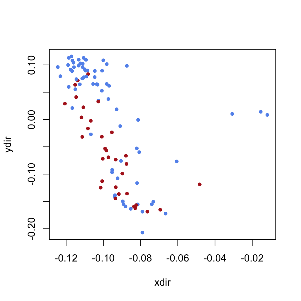
During class, we will talk about how to think about this picture. We will also compare this plot to plots made using the other eigenvectors.
23.3.3 Creating a Table Sorted by an Eigenvector
When we get to more contemporary data, it will be fun later on to look at the names of the Senators who get large (positive or negative) eigenvector scores. Here is some code to help with that.
myorder= order(v1)

eigendata = data.frame(cbind(v1,v2, sen.party))
rownames(eigendata)=sen.name


myorder= order(v1)

knitr::kable(
  head(eigendata[myorder,]), booktabs = TRUE,
  caption = 'One Extreme'
)| v1 | v2 | sen.party | |
|---|---|---|---|
| INOUYE Daniel Ken | -0.124510990388193 | 0.0960716902237526 | D |
| McINTYRE Thomas James | -0.123097587465213 | 0.0793272186071726 | D |
| SMITH Margaret Chase | -0.120654354853401 | 0.0290668793843522 | R |
| MUSKIE Edmund Sixtus | -0.118947766632202 | 0.0997692334878442 | D |
| MONRONEY Almer Stillwell Mike | -0.118641982145802 | 0.0596868115454118 | D |
| HUMPHREY Hubert Horatio Jr. | -0.118613491347109 | 0.112820684546629 | D |
myrevorder = order(-v1)

knitr::kable(
  head(eigendata[myrevorder,]), booktabs = TRUE,
  caption = 'The Other Extreme'
)| v1 | v2 | sen.party | |
|---|---|---|---|
| SALINGER Pierre Emil George | -0.011895821132766 | 0.00841073422406016 | D |
| KEFAUVER Carey Estes | -0.0154423731600536 | 0.0140931934686823 | D |
| ENGLE Clair | -0.0307343177099913 | 0.0102249015658184 | D |
| GOLDWATER Barry Morris | -0.0482357085359829 | -0.118817158736983 | R |
| WALTERS Herbert Sanford | -0.0605618365871763 | -0.0767520789280585 | D |
| BYRD Harry Flood | -0.0665699568843238 | -0.172435813910847 | D |
23.4 Your Turn
The data for the 88th Congressional Session (1964) does not seem very partisan. Democrats and Republicans are finding plenty of common ground. When we look at the “extremes” we find some recognizable names, including Hubert Humphrey (D) and Barry Goldwater (R). But there is no clear “left” or “right” pattern to the party affiliation.
What about the remaining 5 data sets? It’s your turn to explore and discuss.
The code above has been written for ease of reuse.
- Go back to the top and change the following line:
# pick the data set that we want to look at
senate.files = senate.1964.files
to one of the other options: senate.1976.files, senate.1988.files, senate.2000.files, senate.2012.files
Do a similar analysis as described above, as well as the things we tried in class together.
- Find the eigenvalues. Where are the gaps? What is the rough “dimension” of each data set?
- Plotting the two dominant eigenvectors. Do you see evidence of political divission?
- Then try plotting other pairs of eigenvectors. Which ones are just noise?
- Create tables of the two extreme for the dominant eigenvectors. Do you see any names that you recognize?
Finally, you have some evidence to help you to answer the orignal question: “Is US Politics more polarized than ever before?”