Vector 1 Problem Set 1
- Due: Tuesday November 3 by 11:55pm CST.
- Upload your solutions to Moodle in a PDF.
- Please feel free to use RStudio for all row reductions.
- You can download the Rmd source file for this problem set.
1.1 Characterize the Solution Set
The following augmented matrices are in row echelon form. Decide whether the set of solutions is a point, line, plane, or the empty set in 3-space. Briefly justify your answer.
\(\left[ \begin{array}{ccc|c} 1 & 3 & -1 & 4 \\ 0 & 1 & 4 & 0\\ 0 & 0 & 0 & 2 \\ \end{array} \right]\)
\(\left[ \begin{array}{ccc|c} 1 & 3 & -1 & 5 \\ 0 & 0 & 0 & 0 \\ 0 & 0 & 0 & 0 \\ \end{array} \right]\)
\(\left[ \begin{array}{ccc|c} 1 & -1 & 0 & -2 \\ 0 & 0 & 1 & 7\\ 0 & 0 & 0 & 1\\ \end{array} \right]\)
\(\left[ \begin{array}{ccc|c} 0 & 1 & 0 & 6 \\ 0 & 0 & 1 & -2 \\ 0 & 0 & 0 & 0 \\ \end{array} \right]\)
1.2 Find the Parametric Solution
Each of the following matrices is the reduced row echelon form of the augmented matrix of a system of linear equations. Give the general solution to each system.
\(\left[ \begin{array}{cccc|c} 1 & 3 & 0 & -2 & 5\\ 0 & 0 & 1 & 4 & -2 \\ \end{array} \right]\)
\(\left[ \begin{array}{ccccc|c} 1 & 0 & 4 & 0 & 3 & 6\\ 0 & 1 & 1 & 0 & -2& -8 \\ 0 & 0 & 0 & 1 & -1 & 3 \\ \end{array} \right]\)
\(\left[ \begin{array}{cccc|c} 1 & 4 & 0 & 0 & -2 \\ 0 & 0 & 1 & 7 & 6\\ 0 & 0 & 0 & 0 & 0 \\ \end{array} \right]\)
1.3 Elementary row operations are reversible
In each case below, an elementary row operation turns the matrix \(A\) into the matrix \(B\). For each of them,
- Describe the row operation that turns \(A\) into \(B\), and
- Describe the row operation that turns \(B\) into \(A\).
Give your answers in the form: “scale \(R_2\) by 3” or “swap \(R_1\) and \(R_4\)” or “replace \(R_3\) with \(R_3 + \frac{1}{5} R_1\).”
\[A=\left[ \begin{array}{cccc} 1 & 1 & 1 & 3 \\ 1 & -2 & 2 & 1 \\ 2 & 8 & 2 & -4 \\ 3 & 1 & 6 & -1 \\ \end{array} \right]\longrightarrow B=\left[ \begin{array}{cccc} 1 & 1 & 1 & 3 \\ 1 & -2 & 2 & 1 \\ 2 & 8 & 2 & -4 \\ 0 & 7 & 0 & -4 \\ \end{array} \right]\]
\[A=\left[ \begin{array}{cccc} 1 & 1 & 1 & 3 \\ 1 & -2 & 2 & 1 \\ 2 & 8 & 2 & -4 \\ 3 & 1 & 6 & -1 \\ \end{array} \right]\longrightarrow B=\left[ \begin{array}{cccc} 1 & -2 & 2 & 1 \\ 1 & 1 & 1 & 3 \\ 2 & 8 & 2 & -4 \\ 3 & 1 & 6 & -1 \\ \end{array} \right]\]
\[A=\left[ \begin{array}{cccc} 1 & 1 & 1 & 3 \\ 1 & -2 & 2 & 1 \\ 2 & 8 & 2 & -4 \\ 3 & 1 & 6 & -1 \\ \end{array} \right]\longrightarrow B=\left[ \begin{array}{cccc} 1 & 1 & 1 & 3 \\ 1 & -2 & 2 & 1 \\ 1 & 4 & 1 & -2 \\ 3 & 1 & 6 & -1 \\ \end{array} \right]\]
1.4 Traffic Flow
Below you find a section of one-way streets in downtown St Paul, where the arrows indicate traffic direction. The traffic control center has installed electronic sensors that count the numbers of vehicles passing through the 6 streets that lead into and out of this area. Assume that the total flow that enters each intersection equals the the total flow that leaves each intersection (we will ignore parking and staying).
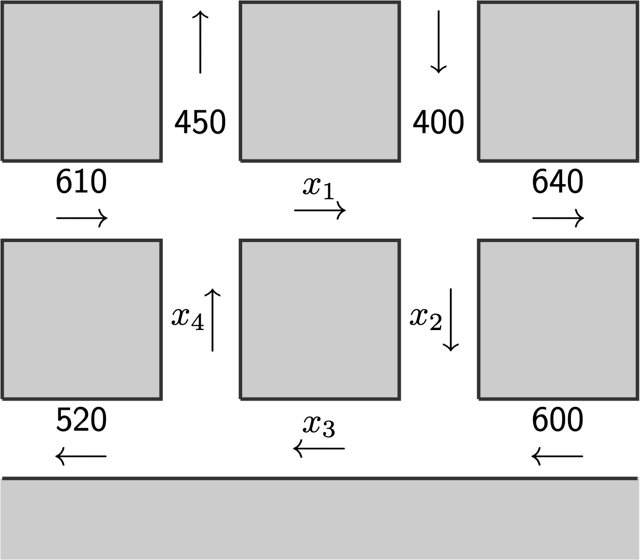
Create a system of linear equations to find the possible flow values for the inner streets \(x_1, x_2, x_3, x_4\).
Use RStudio to find the solution set. Write your answer in parametric form.
Your answer to part 2 finds an infinite solution set. In terms of traffic flow, explain why there can be more than one solution. Thinking about cars traveling along streets, why is there some flexibility in the overall flow of cars?
Now critique the model as presented. What solutions to the linear system are problematic for our original traffic flow problem? What additional conditions should we require for a valid solution?
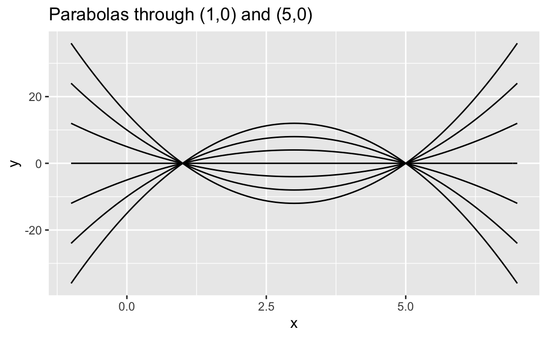
1.5 Parabolas Through Two Points
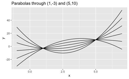
You will find the family of all possible parabolas \[ f(x) = a x^2 + b x + c \] through two given points. Note that there will be an infinite number of such polynomials: there are three unknowns, but only two constraints. So there will be at least one free variable. Here are the plots of the two different families of parabolas that you will consider.
For each pair of points below:
- Create linear system that represents the problem
- Use RStudio to find the RREF of the augmented matrix for the system and
- Write down the general formula for the family of parabolas \(f(x)\) that contain the points.
Here are the pairs of points.
\(p_1 = (1,0)\) and \(p_2 = (5,0)\)
\(q_1= (1,-3)\) and \(q_2 = (5,10)\)
Part (a.i) characterizes the family of parabolas that contain the points \(p_1\) and \(p_2\). Let’s refer to this family of parabolas as our “\(p_1,p_2\) family.” Pick any two functions \(g_1(x)\) and \(g_2(x)\) from this \(p_1,p_2\) family of parabolas. Now consider the parabola \[ g(x) = g_1(x) - g_2(x). \] Show that \(g(1)=0\) and \(g(5)=0\). This means that \(g(x)\) is also in our \(p_1,p_2\) family! (That’s really cool!)
Part (a.ii) characterizes the family of parabolas that contain the points \(q_1\) and \(q_2\). Let’s refer to this family of parabolas as our “\(q_1,q_2\) family.” Pick any two functions \(h_1(x)\) and \(h_2(x)\) in this \(q_1,q_2\) family. Now consider the parabola \[ h(x) = h_1(x) - h_2(x). \] Show that \(h(1) \neq -3\) and \(h(5) \neq 10\). This means that \(h(x)\) is NOT in our \(q_1,q_2\) family. (So this family is not as nice as the previous one.)
Now explain why the parabola \(h(x)\) from part 3 is actually a member of the \(p_1, p_2\) family. (So maybe this family is nicer than we thought!)
Remark: This problem is about families of parabolas. But at its core, this is actually a problem about linear algebra.
- Obviously, we used linear algebra to solve part 1, but there is linear algebra in the other parts as well!
- We define \(g(x) = g_1(x) - g_2(x)\) by taking a linear combination of two functions. (Just like we take linear combinations of vectors.)
- What leads to the “nice” behavior of the \(p_1, p_2\) family in part 2? It’s because the \(y\)-values of the constraining points are both 0. We will soon learn about homogeneous linear systems whose right hand sides are all zero. These homogeneous systems have some very special properties.
- The \(q_1, q_2\) family is “not nice” because it a nonhomogenous system.
- Just as there is a connection betwen the \(p_1,p_2\) family and the \(q_1, q_2\) family, we will soon learn that there is a connection between homogeneous systems and nonhomogeneous systems.