Vector 31 Quiz 4 Review

31.1 Overview

Our fourth quiz covers sections 6.1-6.5, 7.1 and 7.4 in Lay’s book. This corresponds to Problem Set 8.

The best way to study is to do practice problems. The Quiz will have calculation problems (like Edfinity) and more conceptual problems (like the problem sets). Here are some ways to practice:

Make sure that you have mastered the Vocabulary, Skills and Concepts listed below.
Look over the Edfinity homework assingments
Do practice problems from the Edfinity Practice assignments. These allow you to “Practice Similar” by generating new variations of the same problem.
Redo the Jamboard problems
Try to resolve the Problem Sets and compare your answers to the solutions.
Do the practice problems below. Compare your answers to the solutions.

31.1.1 Vocabulary, Concepts and Skills

See the Week 7-8 Learning Goals for the list of vocabulary, concepts and skills.

31.2 Practice Problems

31.2.1

Let \(\mathsf{v} = \begin{bmatrix}1 \\ -1 \\ 1 \end{bmatrix}\) and \(\mathsf{w}= \begin{bmatrix}5 \\ 2 \\ 3 \end{bmatrix}\).

Find \(\| \mathsf{v} \|\) and \(\| \mathsf{w} \|\).
Find the distance between \(\mathsf{v}\) and \(\mathsf{w}\).
Find the cosine of the angle between \(\mathsf{v}\) and \(\mathsf{v}\).
Find \(\mbox{proj}_{\mathsf{v}} \mathsf{w}\).
Let \(W=\mbox{span} (\mathsf{v}, \mathsf{w})\). Create an orthonormal basis \(\mathsf{u}_1, \mathsf{u}_2\) for \(W\) such that \(\mathsf{u}_1\) is a vector in the same direction as \(\mathsf{v}\).

31.2.2

Let \(\mathsf{u} \neq 0\) be a vector in \(\mathbb{R}^n\). Define the function \(T: \mathbb{R}^n \rightarrow \mathbb{R}^n\) by \(T(\mathsf{x}) = \mbox{proj}_{\mathsf{u}} \mathsf{x}\).

Prove that \(T: \mathbb{R}^n \rightarrow \mathbb{R}^n\) is a linear transformation.
Recall that the kernel of \(T\) is the subspace \(\mbox{ker}(T) = \{ \mathsf{x} \in \mathbb{R}^n \mid T(x) = \mathbf{0} \}\). Describe \(\mbox{ker}(T)\) as explicitly as you can.

31.2.3

The vectors \(\mathsf{u}_1, \mathsf{u}_2\) form an orthonormal basis of a subspace \(W\) of \(\mathbb{R}^4\). Find the projection of \(\mathsf{v}\) onto \(W\) and determine how close \(\mathsf{v}\) is to \(W\). \[ \mathsf{u}_1 = \frac{1}{2}\begin{bmatrix} 1\\ -1\\ -1\\ 1 \end{bmatrix}, \quad \mathsf{u}_2 = \frac{1}{2}\begin{bmatrix} 1\\ -1\\ 1\\ -1 \end{bmatrix}, \quad \mathsf{v} = \begin{bmatrix} 2\\ 2\\ 4\\ 2 \end{bmatrix} \]

31.2.4

Consider vectors \(\mathsf{v}_1 = \begin{bmatrix} 1 \\ 1 \\-1 \end{bmatrix}\) and \(\mathsf{v}_2= \begin{bmatrix} 1 \\ 2 \\ 3 \end{bmatrix}\) in \(\mathbb{R}^3\). Let \(W=\mbox{span}(\mathsf{v}_1, \mathsf{v}_2)\).

Show that \(\mathsf{v}_1\) and \(\mathsf{v}_2\) are orthogonal.
Find a basis for \(W^{\perp}\).
Use orthogonal projections to find the representation of \(\mathsf{y} = \begin{bmatrix} 8 \\ 0 \\ 2 \end{bmatrix}\) as \(\mathsf{y} = \hat{\mathsf{y}} + \mathsf{z}\) where \(\hat{\mathsf{y}} \in W\) and \(\mathsf{z} \in W^{\perp}\).

31.2.5

Let \(W\) be the span of the vectors \[ \begin{bmatrix} 1 \\ -2 \\ 1 \\ 0 \\1 \end{bmatrix}, \quad \begin{bmatrix} -1 \\ 3 \\ -1 \\ 1 \\ -1 \end{bmatrix}, \quad \begin{bmatrix} 0 \\ 0 \\ 1 \\ 3 \\1 \end{bmatrix}, \quad \begin{bmatrix} 0 \\ 2 \\ 0 \\ 0 \\4 \end{bmatrix} \]

Find a basis for \(W\). What is the dimension of this subspace?
Use the Gram-Schmidt process on your answer to part (a) to find an orthonormal basis for \(W\)
Find a basis for \(W^{\perp}\)
Use the Gram-Schmidt process on your answer from part (c) to find an orthogonal basis for \(W^{\perp}\).

31.2.6

Let \(\mathsf{u}_1, \mathsf{u}_1, \ldots, \mathsf{u}_n\) be an orthonormal basis for \(\mathbb{R}^n\). Pick any \(\mathsf{v} \in \mathbb{R}^n\). Show that \[ \| \mathsf{v} \| = \sqrt{ ( \mathsf{v} \cdot \mathsf{u}_1)^2 + (\mathsf{v} \cdot \mathsf{u}_2)^2 + \cdots +(\mathsf{v} \cdot \mathsf{u}_n)^2}. \]

31.2.7

Consider the system \(A \mathsf{x} = \mathsf{b}\) given by \[ \begin{bmatrix} 1 & 1 & 1 \\ 1 & 2 & -1 \\ 1 & 1 & -1 \\ 1 & 2 & 1 \end{bmatrix} \begin{bmatrix} x_1\\ x_2 \\ x_3 \end{bmatrix} = \begin{bmatrix} 4\\ 1 \\ -2 \\ -1 \end{bmatrix}. \]

Show that this system is inconsistent.
Find the projected value \(\hat{\mathsf{b}}\), and the residual \(\mathsf{z}\).
How close is your approximate solution to the desired target vector?

31.2.8

According to the COVID Tracking Project, Minnesota had \(54,463\) positive COVID-19 cases between March 6 and 31 July, 2020. As of 16 December, 2020, that count has reached \(386,412\).

The vector covid.mn lists the total number of new COVID-19 cases in Minnesota between August 1, 2020 and December 16, 2020 (on top of the previously reported \(54,463\)).

covid.start = 54463

covid.mn = c(725, 1484, 2097, 2699, 3316, 4177, 4722, 5638, 6435, 7053, 7376, 7840, 8530, 9260, 9950, 10689, 11253, 11598, 12155, 12845, 13670, 14404, 15121, 15835, 16244, 16773, 17927, 18777, 19794, 20726, 21401, 21892, 22622, 23660, 24503, 25417, 26124, 26762, 27145, 27405, 27786, 28253, 29125, 29848, 30486, 30888, 31350, 32259, 33344, 34258, 35554, 36479, 36959, 37637, 38549, 39726, 41196, 42271, 43175, 43984, 44671, 45737, 46903, 48324, 49363, 50336, 51277, 52188, 53459, 54849, 56365, 57805, 58976, 60111, 61480, 62643, 64933, 66627, 68349, 69976, 71068, 72128, 73689, 75400, 77659, 79339, 80909, 83073, 84981, 87848, 91002, 94009, 96209, 99157, 102633, 106460, 110402, 115844, 120491, 126399, 130325, 135218, 140107, 147332, 152876, 161565, 169118, 176555, 182486, 187580, 195443, 202237, 208489, 215694, 222037, 228453, 234840, 234840, 240538, 249560, 258506, 264300, 267849, 273014, 279163, 284510, 290818, 296399, 301689, 304740, 309256, 312755, 316505, 320935, 324360, 327378, 329701, 331949)

Find the best fitting exponential function \(f(t) = a e^{k t}\) for the number of COVID-19 cases in Minnesota since 31 July, 2020. Here \(t\) is the number of days since 31 July.
Run the following code to plot your function. This code assumes that your least squares solution is given by xhat. Does it look like a good fit?

a = exp(xhat[1])
k = xhat[2]

f=function(y){a * exp(k*(y))}

plot(x,f(x)+ covid.start,type="l",lwd=3,ylab="new positive COVID-19 cases", xlab="days since July 31, 2020", main="best fit exponential function")
points(x,covid.mn + covid.start,pch=20,cex=.7,col="red")

31.2.9

Consider the symmetric matrix \[A = \begin{bmatrix} 3 & 0 & 34 & 3 \\ 0 & 6 & -34 & 0 \\ 34 & -34 & 74 & 34 \\ 3 & 0 & 34 & 3 \end{bmatrix} \] a. Use RStudio to find the eigenvalues \(\lambda_1 > \lambda_2 > \lambda_3 > \lambda_4\) and their corresponding eigenvectors \(\mathsf{v}_1, \mathsf{v}_2, \mathsf{v}_3, \mathsf{v}_3\). Confirm that these eigenvectors form an orthonormal set.

Is the linear transformation \(T(\mathsf{x}) = Ax\) invertible? How do you know?
Confirm that \[ A = \lambda_{1} \mathsf{v}_1 \mathsf{v}_1^{\top} + \lambda_{2} \mathsf{v}_2 \mathsf{v}_2^{\top} + \lambda_{3} \mathsf{v}_3 \mathsf{v}_3^{\top} + \lambda_{4} \mathsf{v}_4 \mathsf{v}_4^{\top}. \]
Use your answer in part (d) to find the best rank 2 approximation for \(A\). (Be careful!)

31.2.10

The matrix \[ A = \left[ \begin{array}{cccc} 1 & 2 & 5 \\ 2 & 3 & 6 \\ -1 & 2 & 3 \\ -3 & 0 & 1 \\ 1 & 4 & 5 \\ \end{array} \right] \]

has singular value decomposition

\[ \left[ \begin{array}{cccccc} 0.48 & -0.02 & 0.55 & 0.63 & -0.27 \\ 0.61 & -0.24 & 0.32 & -0.63 & 0.27 \\ 0.30 & 0.43 & -0.24 & -0.32 & -0.75 \\ 0.032 & 0.87 & 0.22 & 0.00 & 0.44 \\ 0.56 & -0.01 & -0.70 & 0.32 & 0.31 \\ \end{array} \right] \left[ \begin{array}{cccc} 11.4 & 0 & 0 \\ 0 & 3.60 & 0 \\ 0 & 0 & 1.39 \\ 0 & 0 & 0 \\ 0 & 0 & 0 \\ \end{array} \right] \left[ \begin{array}{cccc} 0.16 & -0.98 & 0.062 \\ 0.49 & 0.026 & -0.87 \\ 0.86 & 0.17 & 0.49 \\ \end{array} \right]. \]

Find an orthonormal basis for each of the four fundamental subspaces \(\mbox{Nul}(A), \mbox{Col}(A), \mbox{Row}(A), \mbox{Nul}(A^{\top})\).
Confirm that your basis for \(\mbox{Nul}(A)\) is orthogonal to your basis for \(\mbox{Row}(A)\)
Explain how we know that the mapping \(T(\mathsf{x}) = A\mathsf{x}\) is one-to-one.
Since the mapping \(T: \mathbb{R}^3 \rightarrow \mathbb{R}^5\) is one-to-one. It maps a cube in \(\mathbb{R}^3\) to a 3D “retangular cuboid” in \(\mathbb{R}^5\). Does the 3D volume expand, contract, or stay constant after the mapping? How do you know?
What is the best rank 1 approximation of the matrix \(A\)?

31.2.11

Here is a matrix \(A\) and its reduced row echelon form \(B\) \[ A = \begin{bmatrix} 1 & 3 & -3 & 1 & 0 \\ 2 & 1 & 0 & 6 & 5 \\ 3 & 3 & -3 & 6 & 3 \\ -1 & 4 & -3 & -3 & -1 \end{bmatrix} \qquad \longrightarrow \qquad B = \begin{bmatrix} 1 & 0 & 0 & 2.5 & 1.5 \\ 0 & 1 & 0 & 1.0 & 2.0 \\ 0 & 0 & 1 & 1.5 & 2.5 \\ 0 & 0 & 0 & 0.0 & 0.0 \end{bmatrix}. \]

Find a basis for \(\mbox{Nul}(A)\) and \(\mbox{Col}(A)\).
Is the linear transformation \(T(\mathsf{x}) = A \mathsf{x}\) one-to-one? Onto?
How is the SVD for \(A\) related to the SVD for \(B\)? What properties will they share? What properties will be different? Make some conjectures.
Now find the SVD of both \(A\) and \(B\), and test your conjectures. Compare the singular values, the right singular vectors and the left singular vectors. Be sure to compare each of the four fundamental subspaces: \(\mbox{Nul}(M), \mbox{Col}(M), \mbox{Row}(M), \mbox{Nul}(M^{\top})\).

31.2.12

Singular value decomposition can be used for clustering of high dimensional data. Indeed, the singular vectors encode the patterns in a matrix. So let’s try this out on the Senate votes from the 109th Congress (from Problem Set 8). Let’s load in the data and assign a color to each senator according to their party.

library(readr)

senate.vote.file = "https://raw.github.com/mathbeveridge/math236_f20//main/data/SenateVoting109.csv"

senators <- read_csv(senate.vote.file, col_names = TRUE)

## Rows: 99 Columns: 49
## ── Column specification ────────────────────────────────────────
## Delimiter: ","
## chr  (3): Name, Party, State
## dbl (46): V01, V02, V03, V04, V05, V06, V07, V08, V09, V10, ...
## 
## ℹ Use `spec()` to retrieve the full column specification for this data.
## ℹ Specify the column types or set `show_col_types = FALSE` to quiet this message.

sen.mat <- as.matrix(senators[4:49])

sen.color=rep("goldenrod", dim(senators)[1])
sen.color[senators$Party=='D']="cornflowerblue"
sen.color[senators$Party=='R']="firebrick"

Find the singular value decomposition. Define singval to be the singular values. Plot them using the command plot(singval,pch=19,cex=.5,col='blue'). How many “important” singular values are there?
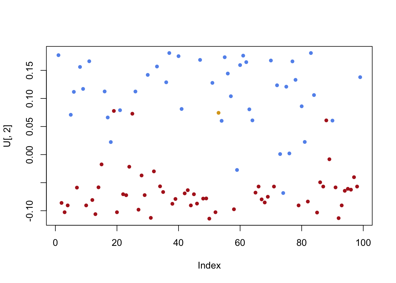
Define U to be the matrix of left singular vectors. Plot the important singular vectors one by one. Here is a command to plot the first singular vector: `plot(U[,1],pch=19,cex=.75,col=sen.color). Do any of the singular values distinguish Democrats from Republicans along the \(y\)-axis?

Remark: When we explored Voting Patterns in the US Senate, we were actually using singular value decomposition to explore those other datasets. In this problem, you looked at a rectangular matrix \(A\) for senators (rows) and votes (columns). In the previous exploration, you were given a square matrix that was (essentially) \(AA^{\top} = (A^{\top}A)^{\top}\). So the eigenvectors of that square matrix are the singular values of the rectangular matrix \(A\).

31.3 Solutions to Practice Problems

31.3.1

\[\begin{align} \| \mathsf{v} \| &= \sqrt{ \mathsf{v} \cdot \mathsf{v}} = \sqrt{1+1+1} = \sqrt{3} \\ \| \mathsf{w} \| &= \sqrt{ \mathsf{w} \cdot \mathsf{vw}} = \sqrt{25+4+9} = \sqrt{38} \\ \end{align}\]
We have \(\mathsf{v} - \mathsf{w} = \begin{bmatrix} -4 \\ -3 \\ -2 \end{bmatrix}\) and so \[ \| \mathsf{v} - \mathsf{w}\| = \sqrt{16+9+4} = \sqrt{29} \]
\[ \cos \theta = \frac{\mathsf{v} \cdot \mathsf{w}}{\| \mathsf{v} \| \, \|\mathsf{w} \| } = \frac{5-2+3}{\sqrt{3} \, \sqrt{38} } = \frac{2\sqrt{3}}{\sqrt{38} } \]
\[ \hat{\mathsf{w}} = \mbox{proj}_{\mathsf{v}} \mathsf{w} = \frac{\mathsf{v} \cdot \mathsf{w}}{ \mathsf{v} \cdot \mathsf{v} } \, \mathsf{v} = \frac{5-2+3}{1+1+1} \mathsf{v} = 2 \mathsf{v} = \begin{bmatrix} 2 \\ -2 \\ 2 \end{bmatrix} \]
Using \(\hat{\mathsf{w}}\) from the previous problem, we know that \[ \mathsf{z} = \mathsf{w} - \hat{\mathsf{w}} = \begin{bmatrix} 5 \\ 2 \\ 3 \end{bmatrix} - \begin{bmatrix} 2 \\ -2 \\ 2 \end{bmatrix} = \begin{bmatrix} 3 \\ 4 \\ 1 \end{bmatrix} \] is orthogonal to \(\mathsf{v}\).So an orthonormal basis is \[ \frac{1}{\sqrt{3}} \begin{bmatrix} 1 \\ -1 \\ 1 \end{bmatrix} \quad \mbox{and} \quad \frac{1}{\sqrt{26}} \begin{bmatrix} 3 \\ 4 \\ 1 \end{bmatrix} \]

31.3.2

We check that \(T(\mathsf{x} + \mathsf{y}) = T(\mathsf{x}) + T(\mathsf{y})\) and that \(T(c\mathsf{x} ) = c \, T(\mathsf{x}).\) To make things a little more clear, let’s write \[ T(\mathsf{x}) = (\mathsf{x} \cdot \mathsf{u}) \, \frac{1}{\mathsf{u} \cdot \mathsf{u}} \mathsf{u} = (\mathsf{x} \cdot \mathsf{u}) \, \frac{1}{\|\mathsf{u} \|^2} \mathsf{u}. \] We have \[\begin{align} T(\mathsf{x} + \mathsf{y}) &= \big((\mathsf{x}+\mathsf{y}) \cdot \mathsf{u} \big) \, \frac{1}{\|\mathsf{u} \|^2} \mathsf{u} = \big(\mathsf{x} \cdot \mathsf{u}+ \mathsf{y} \cdot \mathsf{u} \big) \, \frac{1}{\|\mathsf{u} \|^2} \mathsf{u} \\ &= \big(\mathsf{x} \cdot \mathsf{u} \big) \, \frac{1}{\|\mathsf{u} \|^2} \mathsf{u} + \big(\mathsf{y} \cdot \mathsf{u} \big) \, \frac{1}{\|\mathsf{u} \|^2} \mathsf{u} = T(\mathsf{x}) + T( \mathsf{y}) \end{align}\] and \[ T(c\mathsf{x}) = \big(c\mathsf{x}\cdot \mathsf{u} \big) \, \frac{1}{\|\mathsf{u} \|^2} \mathsf{u} = c \big(\mathsf{x}\cdot \mathsf{u} \big) \, \frac{1}{\|\mathsf{u} \|^2} \mathsf{u} = c \, T(\mathsf{x}) \]
Here are a few ways to describe \(\mbox{ker}(T)\).
- \(\mbox{ker}(T) = \{ \mathsf{x} \in \mathbb{R}^n \mid \mathsf{x} \cdot \mathsf{u} = 0 \}\).
- \(\mbox{ker}(T)\) is the set of vectors that are orthogonal to \(\mathsf{u}\).
- Let \(A\) be the \(1 \times n\) matrix \(\mathsf{u}^{\top}\). Then \(\mbox{ker}(T)= \mbox{Nul}(A)\).

31.3.3

We have \(\mathsf{u}_1 \cdot \mathsf{v} = 2-2-4+2=-2\) and \(\mathsf{u}_1 \cdot \mathsf{v} = 2-2+4-2=2\) so \[ \hat{\mathsf{v}} = \mbox{proj}_W \mathsf{v} = -2 \mathsf{u}_1 + 2 \mathsf{u}_2 = \begin{bmatrix} 1 \\ -1 \\ -1 \\ 1 \end{bmatrix} + \begin{bmatrix} 1 \\ -1 \\ 1 \\ -1 \end{bmatrix} = \begin{bmatrix} 2 \\ -2 \\ 0 \\ 0 \end{bmatrix} \] with residual vector \[ \mathsf{z} = \mathsf{v} - \hat{\mathsf{v}} = \begin{bmatrix} 2 \\ 2 \\ 4 \\ 2 \end{bmatrix} - \begin{bmatrix} 2 \\ -2 \\ 0 \\ 0 \end{bmatrix} = \begin{bmatrix} 0 \\ 6 \\ 4 \\ 2 \end{bmatrix} \] and the distance is \(\| \mathsf{z} \| = \sqrt{36 + 16 + 4} = \sqrt{56}\).

31.3.4

\(\mathsf{v}_1 \cdot \mathsf{v}_2 = 1 +2 - 3 =0\).
We must find \(\mbox{Nul}(A)\) where \(A = \begin{bmatrix} \mathsf{v}_1^{\top} \\ \mathsf{v}_2^{\top}\end{bmatrix}\).

\[ \begin{bmatrix} 1 & 1 & -1 \\ 1 & 2 & 3 \end{bmatrix} \longrightarrow \begin{bmatrix} 1 & 1 & -1 \\ 0 & 1 & 4 \end{bmatrix} \longrightarrow \begin{bmatrix} 1 & 0 & -5 \\ 0 & 1 & 4 \end{bmatrix} \] so the vector \(\begin{bmatrix} 5 \\ -4 \\ 1 \end{bmatrix}\) is a basis for \(W^{\perp}\)

We have \[\begin{align} \hat{\mathsf{y}} &= \frac{\mathsf{y} \cdot \mathsf{v_1}}{\mathsf{v_1} \cdot \mathsf{v_1}} \, \mathsf{v_1} + \frac{\mathsf{y} \cdot \mathsf{v_2}}{\mathsf{v_2} \cdot \mathsf{v_2}} \, \mathsf{v_2} = \frac{8-2}{1+1+1} \mathsf{v_1} + \frac{8+6}{1+4+9} \mathsf{v_2} \\ &= 2\mathsf{v_1} +\mathsf{v_2} = \begin{bmatrix} 2 \\ 2 \\ -2 \end{bmatrix} + \begin{bmatrix} 1 \\ 2 \\ 3 \end{bmatrix} = \begin{bmatrix} 3 \\ 4 \\ 1 \end{bmatrix} \end{align}\] and so \[ \mathsf{z} = \mathsf{y} - \hat{\mathsf{y}} = \begin{bmatrix} 8 \\ 0 \\ 2 \end{bmatrix} - \begin{bmatrix} 3 \\ 4 \\ 1 \end{bmatrix} = \begin{bmatrix} 5 \\ -4 \\ 1 \end{bmatrix}. \]

31.3.5

a .We will answer this one using RStudio.

A = cbind(c(1,-2,1,0,1), c(-1,3,-1,1,-1), c(0,0,1,3,1), c(0,2,0,0,4))
rref(A)

##      [,1] [,2] [,3] [,4]
## [1,]    1    0    0    0
## [2,]    0    1    0    0
## [3,]    0    0    1    0
## [4,]    0    0    0    1
## [5,]    0    0    0    0

So we need all four vectors to span the column space.

RStudio makes this so easy!

gramSchmidt(A)

## $Q
##            [,1]      [,2]          [,3]        [,4]
## [1,]  0.3779645 0.2390457 -8.164966e-01 -0.26233033
## [2,] -0.7559289 0.3585686 -4.082483e-01  0.26233033
## [3,]  0.3779645 0.2390457  2.719480e-16 -0.09837388
## [4,]  0.0000000 0.8366600  4.082483e-01 -0.26233033
## [5,]  0.3779645 0.2390457  2.719480e-16  0.88536488
## 
## $R
##          [,1]      [,2]      [,3]       [,4]
## [1,] 2.645751 -3.401680 0.7559289  0.0000000
## [2,] 0.000000  1.195229 2.9880715  1.6733201
## [3,] 0.000000  0.000000 1.2247449 -0.8164966
## [4,] 0.000000  0.000000 0.0000000  4.0661202

We obtain a basis for \(W^{\perp}\) by finding \(\mbox{Nul(A^{\top})}\) So let’s row reduce \(A^{\top}\)

rref(t(A))

##      [,1] [,2] [,3] [,4] [,5]
## [1,]    1    0    0    0   -2
## [2,]    0    1    0    0    2
## [3,]    0    0    1    0    7
## [4,]    0    0    0    1   -2

The vector \(\begin{bmatrix} 2 \\ -2 \\ -7 \\ 2 \\ 1\end{bmatrix}\) spans \(W^{\perp}\)

Using Gram-Schmidt is overkill for this problem. I’ll just divide by the length of the vector.

vec = c(2,-2,-7,2,1)
vec / Norm(vec)

## [1]  0.2540003 -0.2540003 -0.8890009  0.2540003  0.1270001

31.3.6

We will show that \(\| \mathsf{v} \|^2 = ( \mathsf{v} \cdot \mathsf{u}_1)^2 + (\mathsf{v} \cdot \mathsf{u}_2)^2 + \cdots +(\mathsf{v} \cdot \mathsf{u}_n)^2.\)

Let’s write \(\mathsf{v}\) in terms of the orthonormal basis: \(\mathsf{v} = c_1 \mathsf{u}_1 + c_2 \mathsf{u}_2 + \cdots + c_n \mathsf{u}_n\). We then have

\[\begin{align} \| \mathsf{v} \|^2 &= \mathsf{v} \cdot \mathsf{v} \\ &= (c_1 \mathsf{u}_1 + c_2 \mathsf{u}_2 + \cdots + c_n \mathsf{u}_n) \cdot (c_1 \mathsf{u}_1 + c_2 \mathsf{u}_2 + \cdots + c_n \mathsf{u}_n) \\ &= c_1^2 + c_2 + \cdots + c_n^2 \end{align}\] because \(\mathsf{u}_i \cdot \mathsf{u}_i =1\) and \(\mathsf{u}_i \cdot \mathsf{u}_j=0\) for \(i \neq j\).

Finally, we note that \(\mathsf{v} \cdot \mathsf{u_i} = c_i\) using the same facts about the dot projects for the orthonormal basis. So we have verified the claim above.

31.3.7

A = cbind(c(1,1,1,1), c(1,2,1,2),c(1,-1,-1,1))
b  = c(4,1,-2,-1)
rref(cbind(A,b))

##            b
## [1,] 1 0 0 0
## [2,] 0 1 0 0
## [3,] 0 0 1 0
## [4,] 0 0 0 1

There is a pivot in the last column of this augmented matrix, so this system is inconsistent.

Here is the least squares calculation.

#solve the normal equation
(xhat = solve(t(A) %*% A, t(A) %*% b))

##      [,1]
## [1,]    2
## [2,]   -1
## [3,]    1

# find the projection
(bhat = A %*% xhat)

##               [,1]
## [1,]  2.000000e+00
## [2,] -1.000000e+00
## [3,]  6.661338e-16
## [4,]  1.000000e+00

# find the residual vector
(z = b - bhat)

##      [,1]
## [1,]    2
## [2,]    2
## [3,]   -2
## [4,]   -2

# check that z is orthogonal to Col(A)
t(A) %*% z

##               [,1]
## [1,] -8.881784e-16
## [2,]  0.000000e+00
## [3,]  0.000000e+00

# measure the distance between bhat and b
sqrt( t(z) %*% z)

##      [,1]
## [1,]    4

The projection is \(\hat{\mathsf{b}} = [2,-1,0,1]^{\top}\). The residual is \(\mathsf{z} = [2,2,-2,-2]^{\top}\)

The distance of between \(\mathsf{b}\) and \(\hat{\mathsf{b}}\) is \[ \| = \| \mathsf{z} \| = \sqrt{4+4+4+4} = \sqrt{16} = 4. \] ###

x = 1:length(covid.mn)
y = log(covid.mn)

A = cbind(x^0, x)

(xhat = solve(t(A) %*% A, t(A) %*% y))

##         [,1]
##   8.66588980
## x 0.03138331

a = exp(xhat[1])
k = xhat[2]

f=function(y){a * exp(k*(y))}

plot(x,f(x)+ covid.start,type="l",lwd=3,ylab="new positive COVID-19 cases", xlab="days since July 31, 2020", main="best fit exponential function")
points(x,covid.mn + covid.start,pch=20,cex=.7,col="red")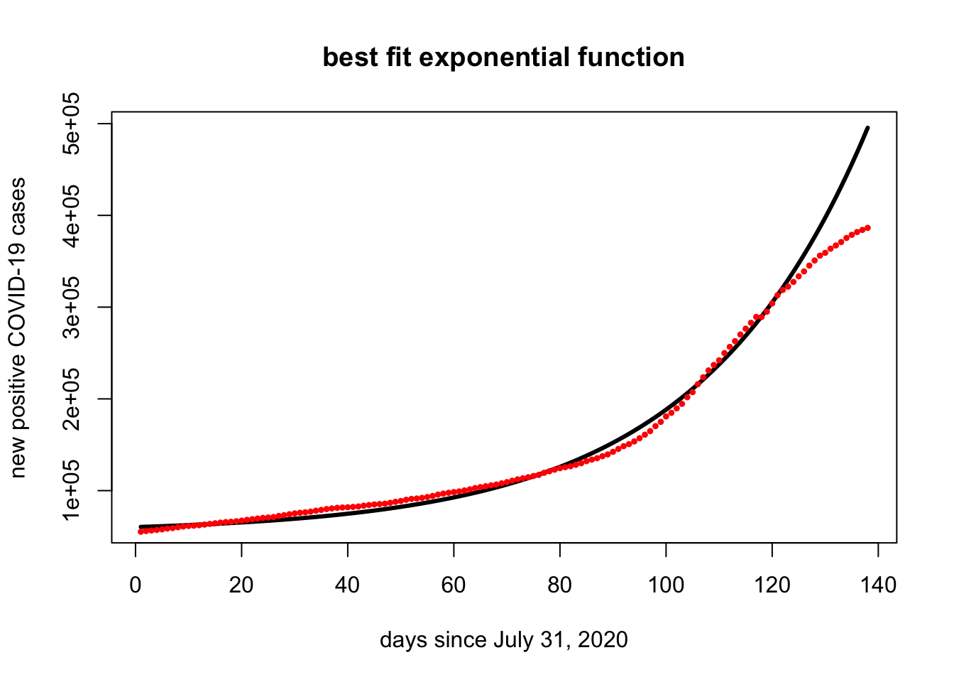

The curve is a pretty good fit (unfortunately?). However, it does look like the additional restrictions of the last two weeks are slowing the COVID spread.

31.3.8

A = cbind(c(3,0,34,3), c(0,6,-34,0), c(34,-34,74,34),c(3,0,34,3))
A

##      [,1] [,2] [,3] [,4]
## [1,]    3    0   34    3
## [2,]    0    6  -34    0
## [3,]   34  -34   74   34
## [4,]    3    0   34    3

syst = eigen(A)

(P = syst$vectors)

##            [,1]          [,2]          [,3] [,4]
## [1,] -0.2886751  4.082483e-01 -7.071068e-01  0.5
## [2,]  0.2886751  8.164966e-01 -3.295975e-15 -0.5
## [3,] -0.8660254 -3.330669e-16  7.771561e-16 -0.5
## [4,] -0.2886751  4.082483e-01  7.071068e-01  0.5

zapsmall(P %*% t(P))

##      [,1] [,2] [,3] [,4]
## [1,]    1    0    0    0
## [2,]    0    1    0    0
## [3,]    0    0    1    0
## [4,]    0    0    0    1

The eigenvectors are the columns of the second matrix \(P\) shown above. The last matrix shows that \(P P^{\top} = I\), so the columns are orthonormal.

## [1] 108   6   0 -28

\(A\) is not invertible because 0 is an eigenvalue.

v1 = syst$vectors[,1]
v2 = syst$vectors[,2]
v3 = syst$vectors[,3]
v4 = syst$vectors[,4]

syst$values[1] * v1 %*% t(v1) + syst$values[2] * v2 %*% t(v2) + syst$values[3] * v3 %*% t(v3) + syst$values[4] * v4 %*% t(v4)

##               [,1]          [,2] [,3]         [,4]
## [1,]  3.000000e+00 -1.776357e-15   34 3.000000e+00
## [2,] -1.776357e-15  6.000000e+00  -34 5.595524e-14
## [3,]  3.400000e+01 -3.400000e+01   74 3.400000e+01
## [4,]  3.000000e+00  5.595524e-14   34 3.000000e+00

We must remember to use the eigenvalues of largest magnitude: these are \(\lambda_1 = 108\) and \(\lambda_4 = -28\).

syst$values[1] * v1 %*% t(v1)  + syst$values[4] * v4 %*% t(v4)

##      [,1] [,2] [,3] [,4]
## [1,]    2   -2   34    2
## [2,]   -2    2  -34   -2
## [3,]   34  -34   74   34
## [4,]    2   -2   34    2

31.3.9

This SVD factorization is \(U \Sigma V^{\top}\).
- \(\mbox{Nul}(A) = \{ 0 \}\) so it has no basis.
- An orthonormal basis for \(\mbox{Col}(A)\) is the first three columns of \(U\).
- An orthonormal basis for \(\mbox{Row}(A)\) is the three rows of \(V^{\top}\). +An orthonormal basis for \(\mbox{Nul}(A^{\top})\) is the last two columns of \(U\).
This is true because the zero vector is orthogonal to every vector.
The matrix \(\Sigma\) has 3 pivots. So the nullspace of \(A\) is trivial.
The 3D volume expands because the product of the singular values is greater than 1.

11.4 * cbind(c(0.48,0.61,0.30,0.032,0.56)) %*% rbind(c(0.16,-0.98,0.062))

##          [,1]      [,2]      [,3]
## [1,] 0.875520 -5.362560 0.3392640
## [2,] 1.112640 -6.814920 0.4311480
## [3,] 0.547200 -3.351600 0.2120400
## [4,] 0.058368 -0.357504 0.0226176
## [5,] 1.021440 -6.256320 0.3958080

31.3.10

The null space is the span of \([-2.5,-1,-1.5,1,0]^{\top}\) and \([-1.5,-2,-2.5,0,1]^{\top}\). The column space is the span of \([1,2,3,-1]^{\top}\) and \([3,1,3,4]^{\top}\) and \([-3,0,-3,-3]^{\top}\)
This mapping is not one-to-one because the null space is two-dimensional. The mapping is not onto because there is no pivot in the final row of \(B\).
This is a conceptual question without a particular “right answer.” Here are some observations.
- The nullspace of \(A\) is the same as the nullspace of \(B\), so an orthogonal basis for \(\mbox{Nul}(A)\) is also an orthogonal basis for \(\mbox{Nul}(B)\). However, the orthonormal basis vector in the SVD for \(A\) do not need to be the same as the orthonormal basis in the SVD for \(B\).
- The columnspace of \(A\) is different from the columnspace of \(B\). However, each of them is three-dimensional.
- The singular values for \(A\) do not need to equal the singular values of \(B\). Row reduction change the determinant of a square matrix. So it is safe to assume that it will have a similar effect on singular values. However, we konw that both will have 3 singular values since \(A\) and \(B\) have the same rank.

A = rbind(c(1,3,-3,1,0),c(2,1,0,6,5),c(3,3,-3,6,3),c(-1,4,-3,-3,-1))
B = rref(A)

A

##      [,1] [,2] [,3] [,4] [,5]
## [1,]    1    3   -3    1    0
## [2,]    2    1    0    6    5
## [3,]    3    3   -3    6    3
## [4,]   -1    4   -3   -3   -1

##      [,1] [,2] [,3] [,4] [,5]
## [1,]    1    0    0  2.5  1.5
## [2,]    0    1    0  1.0  2.0
## [3,]    0    0    1  1.5  2.5
## [4,]    0    0    0  0.0  0.0

(Asvd = svd(A))

## $d
## [1] 1.170522e+01 7.291802e+00 1.953827e+00 1.048298e-15
## 
## $u
##            [,1]       [,2]       [,3]       [,4]
## [1,] -0.2074163 -0.5081310  0.3142951  0.7745967
## [2,] -0.6655245  0.2640904 -0.6485883  0.2581989
## [3,] -0.7060981 -0.2378931  0.4220968 -0.5163978
## [4,]  0.1244229 -0.7845164 -0.5498965 -0.2581989
## 
## $v
##            [,1]        [,2]       [,3]       [,4]
## [1,] -0.3230339  0.01246428  0.4264992 -0.6959338
## [2,] -0.2484683 -0.70106777 -0.3270500  0.2609756
## [3,]  0.2022409  0.62969638 -0.2863539  0.1988388
## [4,] -0.7526916  0.27463749  0.3096671  0.5095232
## [5,] -0.4758851  0.19080183 -0.7302360 -0.3852494

(Bsvd = svd(B))

## $d
## [1] 4.649483 1.543473 1.000000 0.000000
## 
## $u
##           [,1]       [,2]        [,3] [,4]
## [1,] 0.6088198  0.7877604 -0.09365858    0
## [2,] 0.4779319 -0.4584513 -0.74926865    0
## [3,] 0.6331821 -0.4114072  0.65561007    0
## [4,] 0.0000000  0.0000000  0.00000000    1
## 
## $v
##           [,1]       [,2]          [,3]        [,4]
## [1,] 0.1309436  0.5103818 -9.365858e-02 -0.82024886
## [2,] 0.1027925 -0.2970259 -7.492686e-01  0.05990659
## [3,] 0.1361833 -0.2665465  6.556101e-01 -0.04871373
## [4,] 0.6344264  0.5791090  6.938894e-17  0.49438789
## [5,] 0.7424586 -0.4948451 -5.551115e-17 -0.27714724

# check that the singular values are different
Asvd$d

## [1] 1.170522e+01 7.291802e+00 1.953827e+00 1.048298e-15

Bsvd$d

## [1] 4.649483 1.543473 1.000000 0.000000

Arow = Asvd$v[,1:3]
Acol = Asvd$u[,1:3]

Brow = Bsvd$v[,1:3]
Bcol = Bsvd$u[,1:3]

# check that the rowspaces are the same
# this also means that the nullspaces are the same
rref(cbind(Arow, Brow))

##      [,1] [,2] [,3]       [,4] [,5]       [,6]
## [1,]    1    0    0 -0.8711504    0  0.4023226
## [2,]    0    1    0  0.3312215    0  0.9197649
## [3,]    0    0    1 -0.3624766    0 -0.1264565
## [4,]    0    0    0  0.0000000    1  0.1543445
## [5,]    0    0    0  0.0000000    0  0.0000000

rref(cbind(Brow, Arow))

##      [,1] [,2] [,3]       [,4]      [,5] [,6]
## [1,]    1    0    0 -0.8711504 0.3312215    0
## [2,]    0    1    0 -0.3453768 0.1113812    0
## [3,]    0    0    1  0.3490156 0.9369560    0
## [4,]    0    0    0  0.0000000 0.0000000    1
## [5,]    0    0    0  0.0000000 0.0000000    0

# check that the columnspaces are different
rref(cbind(Acol, Bcol))

##      [,1] [,2] [,3] [,4]        [,5]      [,6]
## [1,]    1    0    0    0  2.77467300 -1.955659
## [2,]    0    1    0    0  0.45357378 -1.059136
## [3,]    0    0    1    0 -0.01928201  1.068529
## [4,]    0    0    0    1  2.62771978 -2.255687

31.3.11

decomp = svd(sen.mat)
singval = decomp$d

plot(singval,pch=19,cex=.5,col='blue')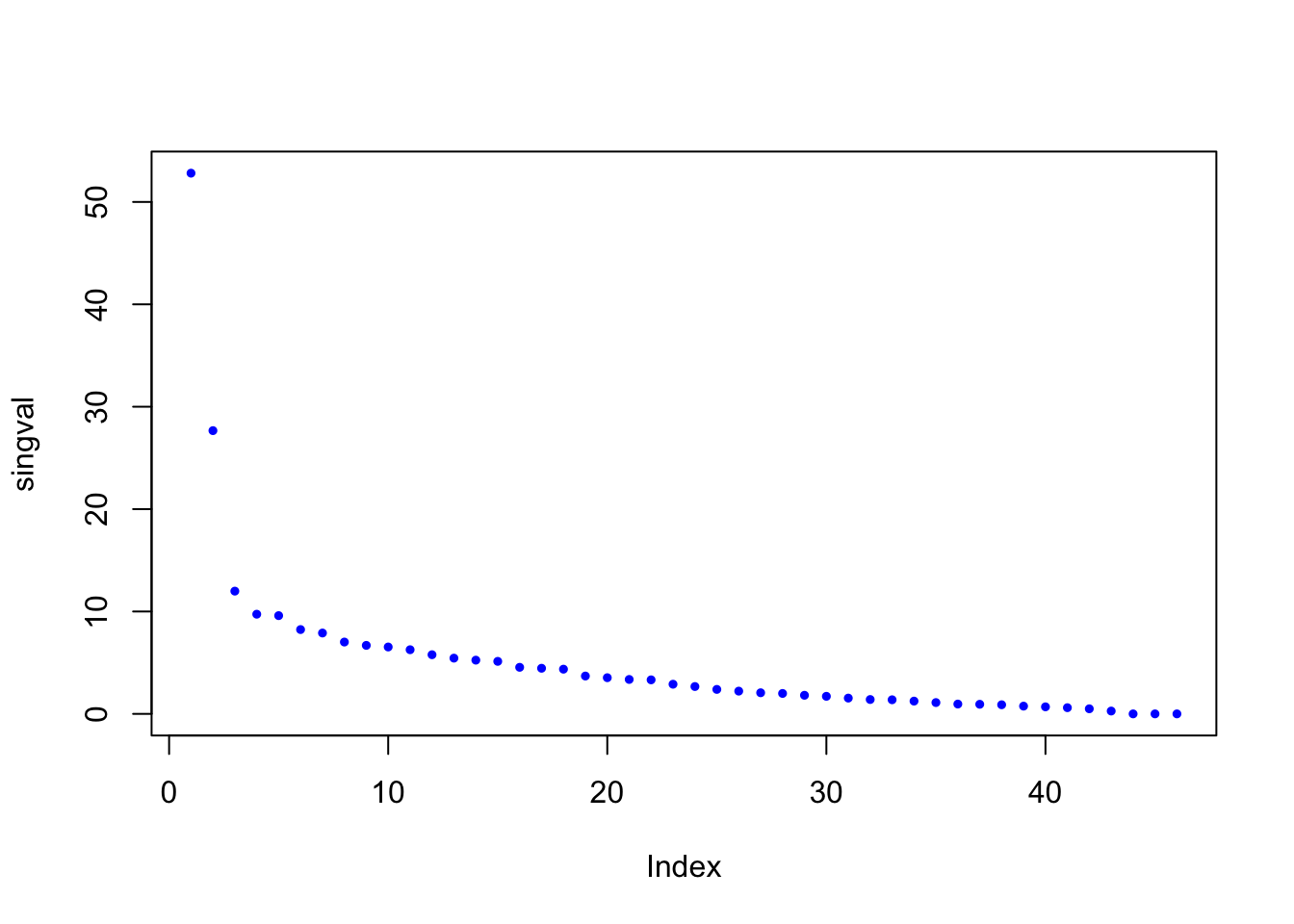

There are two very important eigenvectors. After those two gaps, the eigenvalues taper off more slowly. We certainly need more than the first two for a good approximation of the matrix. But the importance of the rest is more even.

The first left singular vector picks up a mild (but not definitive) layering of Republicans and Democrats. The second left singular vector provides a clear separation!

U = decomp$u

plot(U[,1],pch=19,cex=.75,col=sen.color)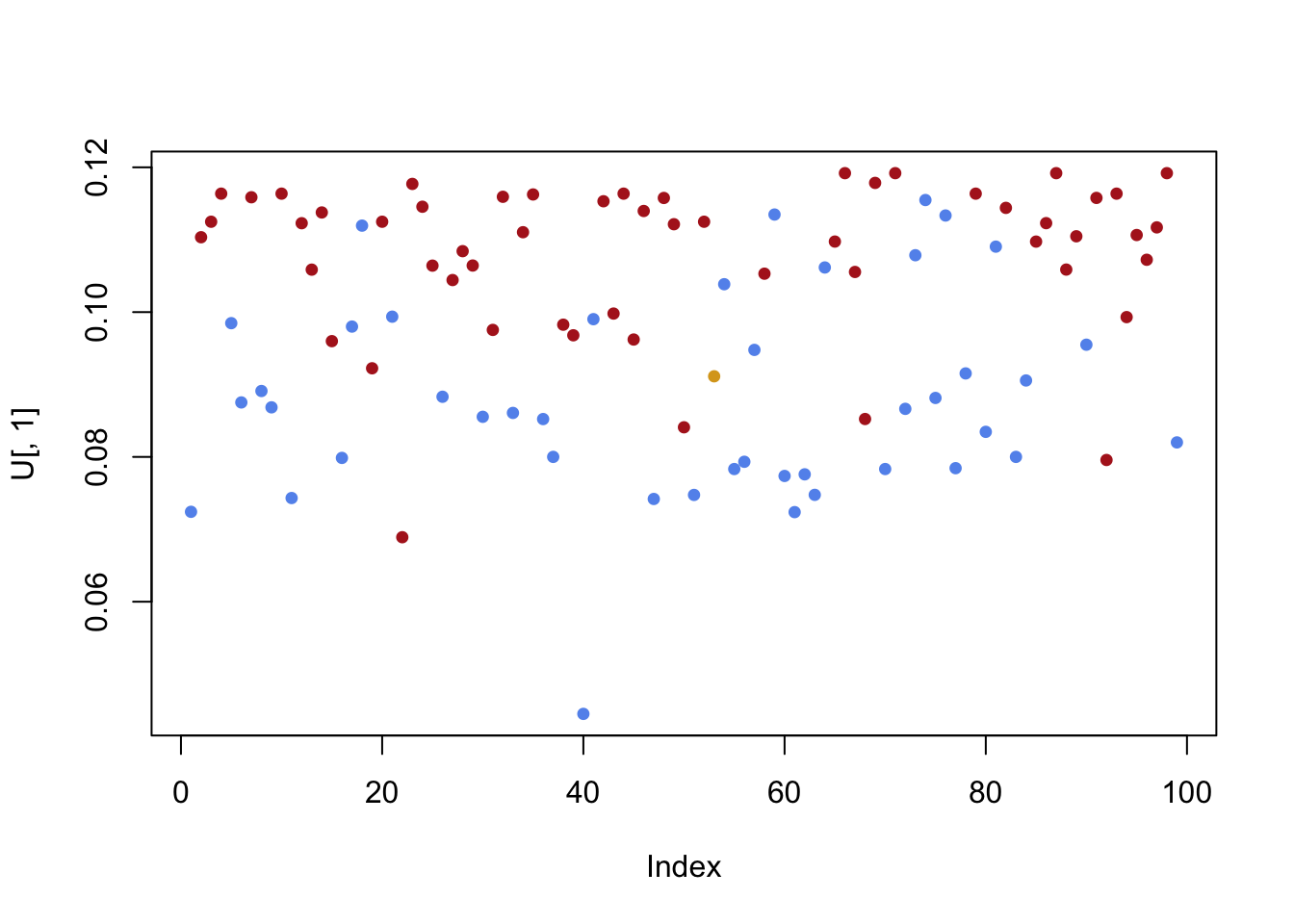

plot(U[,2],pch=19,cex=.75,col=sen.color)