Vector 17 2D Linear Transformations
Let’s explore linear transformations of the plane! Download this Rmd file.
We know that a linear transformation \(T\) satisfies \[ T(c \mathsf{u} + d \mathsf{v}) = c\, T( \mathsf{u}) +d \, T( \mathsf{v}). \] But what do linear transformations look like? Let’s start to answer this question by considering linear transformations of the plane.
We will look at mappings \(T: \mathbb{R}^2 \rightarrow \mathbb{R}^2\) where \(T(\mathsf{x}) = \mathsf{A} \mathsf{x}\) for a \(2 \times 2\) matrix \(\mathsf{A}\). \[ T \left( \begin{bmatrix} x \\ y \end{bmatrix} \right) = \begin{bmatrix} a_{11} & a_{12} \\ a_{21} & a_{22} \end{bmatrix} \begin{bmatrix} x \\ y \end{bmatrix}. \] The linear transformation \(T(\mathsf{x})\) maps the plane to itself. This nicely allows us to compare vectors before the mapping with their images after the mapping. We can then describe the effect of the mapping on the plane.
17.1 Functions to plot our vectors
Here are a couple of helper functions to plot our “before” and “after” vectors as arrows in the plane.
plot_four_vectors <- function(before1, before2, after1, after2){
  a0 = c(0,0, before1[1], before2[1])
  b0 = c(0,0, before1[2], before2[2])
  a1 = c(before1[1],before2[1],before1[1]+before2[1], before1[1]+before2[1])
  b1 = c(before1[2],before2[2],before1[2]+before2[2], before1[2]+before2[2])
  c0 = c(0,0, after1[1], after2[1])
  d0 = c(0,0, after1[2], after2[2])
  c1 = c(after1[1],after2[1],after1[1]+after2[1], after1[1]+after2[1])
  d1 = c(after1[2],after2[2],after1[2]+after2[2], after1[2]+after2[2])
  max_val = max(a0,b0,a1,b1,c0,d0,c1,d1)
  min_val = min(a0,b0,a1,b1,c0,d0,c1,d1)

  plot(NA, xlim=c(min_val*1.5,max_val*1.5), ylim=c(min_val,max_val), xlab="X", ylab="Y", )
  abline(v=0, col="gray")
  abline(h=0, col="gray")
  vecs <- data.frame(vname=c("a","b","a+b", "transb"),
                     x0=a0, y0=b0, x1=a1 ,y1=b1,
                     col=1:4)
  with( vecs, mapply("arrows", x0, y0, x1,y1,col=col, lty=2) )
    vecs <- data.frame(vname=c("a","b","a+b", "transb"),
                     x0=c0, y0=d0, x1=c1, y1=d1,
                     col=1:4)
  with( vecs, mapply("arrows", x0, y0, x1,y1,col=col) )

}
This function has four parameters. The parameters before1 and before2 are two vectors before the mapping, and after1 and after2 are their images after the mapping. The function creates a dashed plot of the parallelogram with corners (0,0), before1, before2 and before1+before2. It also creates a solid plot of the image of this parallelogram. These are plotted on the same plane so taht we can easily compare “before” and “after.”
Here is an example. Let’s start with vectors \(\begin{bmatrix} 3 \\ 0 \end{bmatrix}\) and \(\begin{bmatrix} 0 \\ 2 \end{bmatrix}\). It’s nice to start with vectors of different lengths. Let’s consider the mapping correspoding to multiplication by the matrix
\[
A = \begin{bmatrix} 2 & 3 \\ 4 & -1 \end{bmatrix}.
\]
Here is some example code showing how to make our plot. Note: A %*% x is the syntax for matrix multiplication in R.
vec1 = c(3,0)
vec2 = c(0,2)

A = cbind(c(2,1), c(4,-1))

newvec1 = A %*% vec1
newvec2 = A %*% vec2

plot_four_vectors(vec1, vec2, newvec1, newvec2)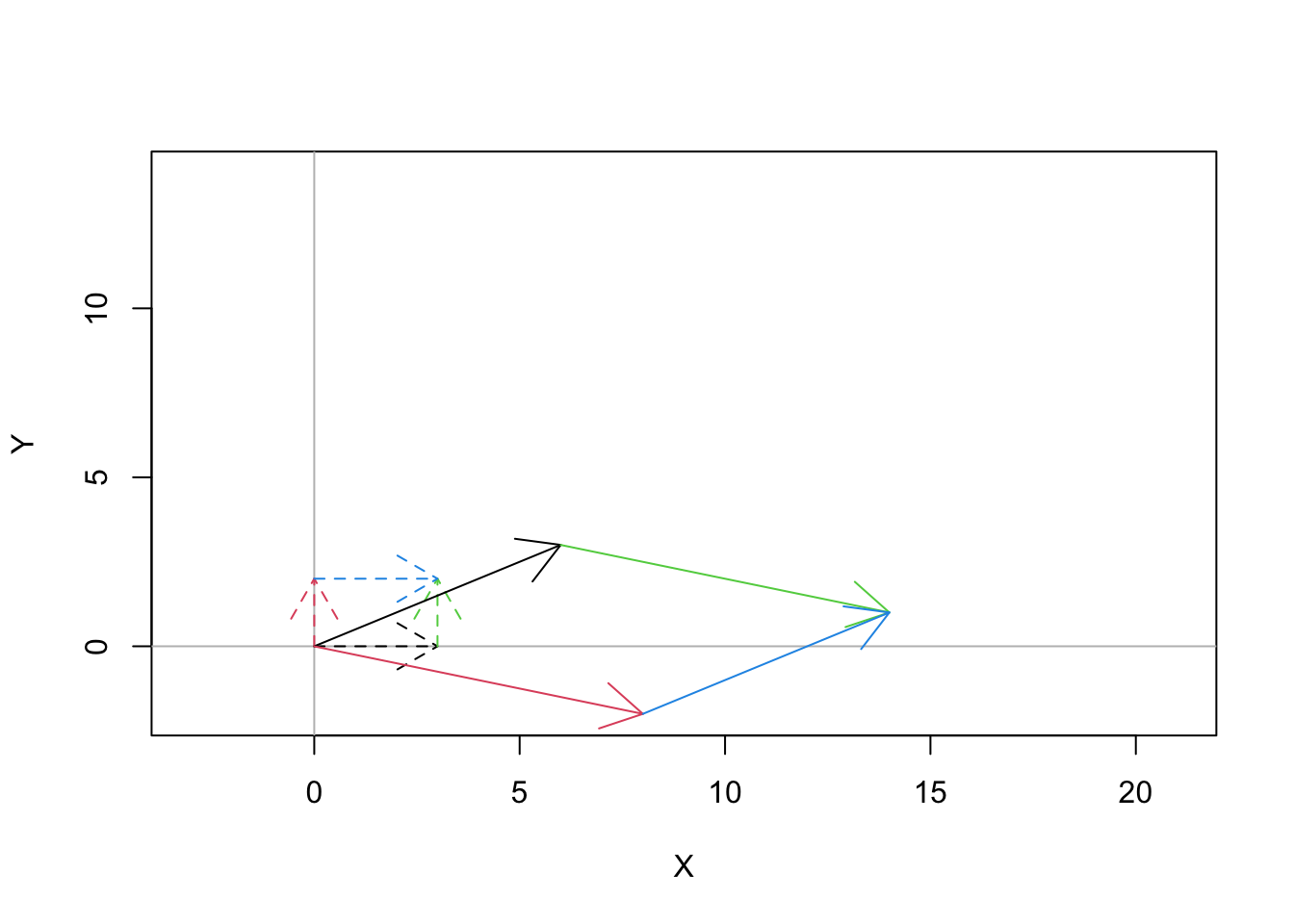
Figure 17.1: An example 2D linear transformation
This visualization uses different colors for the vectors so that you can match up the original vector with its image. There is a lot going on in this mapping, so let’s start making some observations.
- The original rectangle mapped to a parallelogram. So the shape is ``squished’’ a bit.
- Both the black vector and the red vector have gotten larger. But we can see that the red vector has grown much more than the black one. So there is expansion, but it is not uniform.
- The black vector and the red vector have flipped! This means that there is some sort of reflection happening.
There isn’t a simple description for what’s happening here. It’s a combination of effects, so that the image of the rectangle is a warped version of the original.
17.2 Your Turn
Now it’s your turn. Investigate the effect of each of the following families of mappings.
- Using the previous code snippet as a guide, create a “before and after plot” for the black vector \(\begin{bmatrix} 3 \\ 0 \end{bmatrix}\) and the red vector \(\begin{bmatrix} 0 \\ 2 \end{bmatrix}\)
- Describe the effect of the mapping as best you can. Be sure to look at the different effect on the black vector and the red vector. Use words like, expansion, contraction, rotation, reflection and shear.
- Once you have looked at the effect of the family, look back at the form of the matrix \(A\). Can you explain why it leads to the outcome you see?
17.2.1 Family 1
Explore matrices of the form \[A=\displaystyle{ \begin{bmatrix} a & 0 \\ 0 & b \end{bmatrix}}.\] Once again, try various combinations of positive, negative, small and large numbers. Here is some sample code that would create such a matrix for \(a=1\) and \(b=1\).
a = 1
b = 1

A = cbind(c(a,0), c(0,b))
17.2.2 Family 2
Explore matrices of the form \[A=\displaystyle{ \begin{bmatrix} 0 & b \\ c & 0 \end{bmatrix}}.\] Try various combinations of positive and negative numbers. Also try numbers of small magnitude (less than 1) and large magnitude.
17.2.3 Family 3
Explore matrices of the form \[A=\displaystyle{ \begin{bmatrix} \cos(t) & -\sin(t) \\ \sin(t) & \cos(t) \end{bmatrix}}\] where \(t\) is in radians. Here is a function that will create such a matrix.
create_angle_matrix <- function(t) {
  A = cbind(c(cos(t), sin(t)), c(-sin(t), cos(t)))
  return(A)
}

A = create_angle_matrix(pi/2)
A
## [,1] [,2]
## [1,] 6.123234e-17 -1.000000e+00
## [2,] 1.000000e+00 6.123234e-17Note: R is numerical software. You’ll note that sin(pi/2) returns a value of 6.123234e-17 or something similar. This value is given in scientific notation, and is \(\approx 6.12 \times 10^{-17}\). You should treat this tiny number as equal to 0. Be sure to keep an eye out for return values like this that are ``numerically equivalent to 0.’’
17.2.4 Family 4
Now explore matrices of the form \[A=\displaystyle{ \begin{bmatrix} a & -b \\ b & a \end{bmatrix}}\]
Once again, consider a wide variety of such matrices.
17.2.5 Some Other Matrices
Now try these matrices. For each one, try to make other matrices that have a similar effect. (What is the relationship between the entries that leads to this particular kind of image?)
\[ A=\displaystyle{ \begin{bmatrix} 1 & -3 \\ 2 & -6 \end{bmatrix}}, \qquad B=\displaystyle{ \begin{bmatrix} 1 & 1 \\ 0 & 1 \end{bmatrix}}, \qquad C=\displaystyle{ \begin{bmatrix} 0 & 1 \\ 0 & 0 \end{bmatrix}}, \qquad D=\displaystyle{ \begin{bmatrix} 3 & 0 \\ 3 & 2 \end{bmatrix}}, \qquad \]
17.3 Exploration
Now it’s time to explore. Try one or more of the following:
- Can you find a mapping that will turn the rectangle with corners
(0,0), (3,0), (3,2), (0,2)into a square? - Look at some different starting vectors.
- Try some other matrices.
- What is the relationship between the rank of the matrix and the image of the transformation?
17.4 Even More Exploration
For a more interactive experinece, head over to Section 2.6.2 of Understanding Linear Algbra. This short section on the geometry of \(2 \times 2\) matrix transformations has an interactive activity where you can change the entries using slider controls. It is illuminating to see the progressive impact of your choices!