Vector 27 SVD and Image Compression
Today we will use the svd command to find the Singular Value Decomposition of an \(m \times n\) matrix.
We will practice reading the output of this command and finding bases for the four fundamental subspaces of a matrix.
Then we will look at a cool application of SVD: image compression!
27.1 Singular Value Decomposition
Let’s start by looking at the SVD for a couple of matrices. For each one:
- Determine the rank of \(A\)
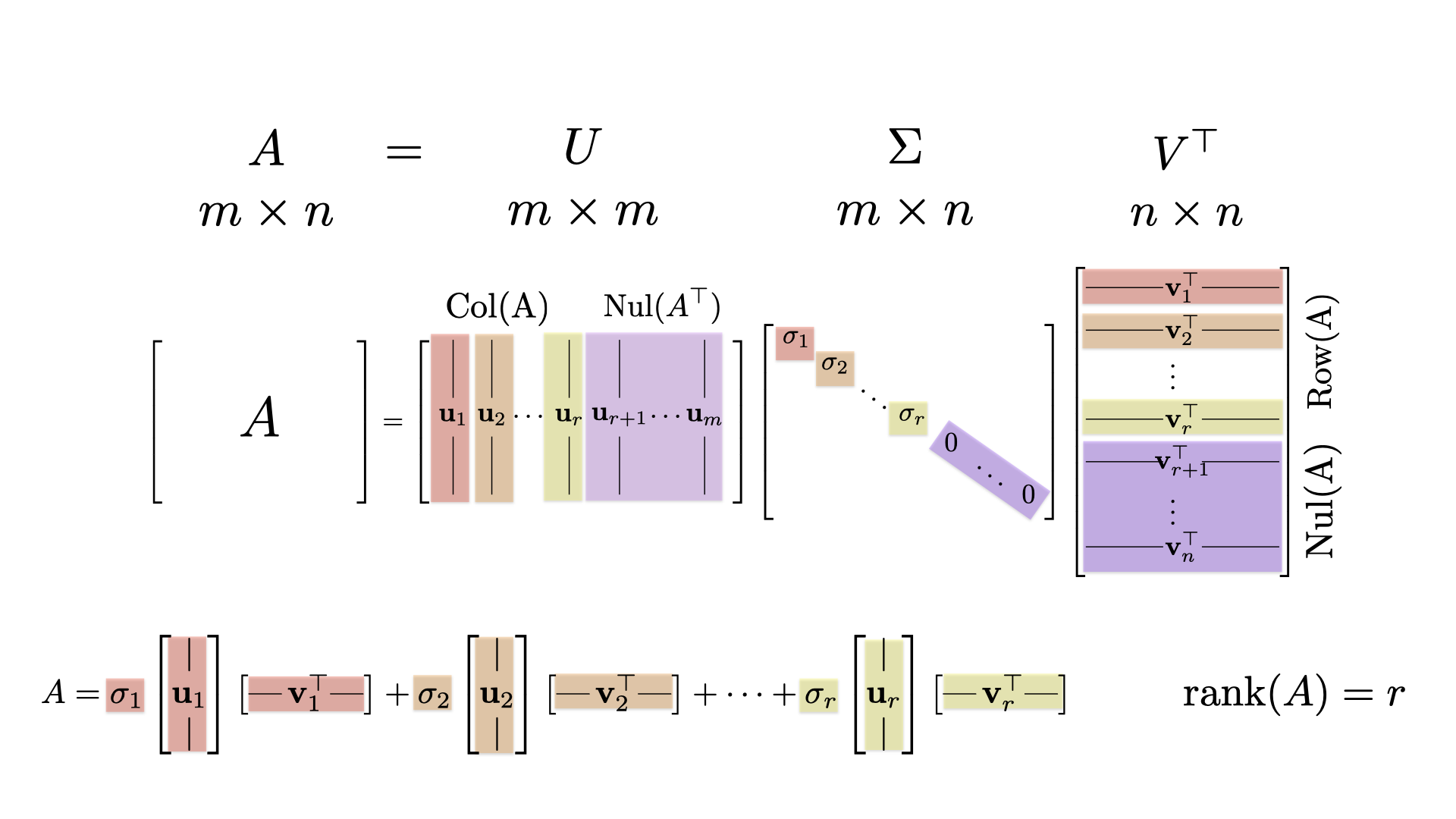
- Identify the basis for each of the four fundamental subspaces \[ \mbox{Nul}(A), \qquad \mbox{Col}(A), \qquad \mbox{Row}(A), \qquad \mbox{Nul}(A^{\top}). \]
- Pick a vector \(\mathsf{x}\) from the basis for \(\mbox{Nul}(A)\) and confirm that \(A \mathsf{x} = \mathbf{0}\).
- Pick a vector \(\mathsf{y}\) from the basis for \(\mbox{Col}(A)\) and confirm that \(\mathsf{y}\) can be written as the a linear combination of the columns of \(A\).
- Find the spectral decomposition of \(A\)
- Use the spectral decomposition to create approximations of matrix \(A\) and then compare the quality of the approximation to the size of the gaps of the singular values.
27.1.1 SVD of a Wide Matrix
Here is a \(4 \times 5\) matrix \(A\).
(A = cbind(c(1,-1,1,0),c(-2,3,0,2),c(1,-1,1,0),c(0,1,4,0),c(1,-1,5,-4)))## [,1] [,2] [,3] [,4] [,5]
## [1,] 1 -2 1 0 1
## [2,] -1 3 -1 1 -1
## [3,] 1 0 1 4 5
## [4,] 0 2 0 0 -4Let’s call svd(A) and see what we get.
(decomp = svd(A))## $d
## [1] 7.657063e+00 4.528454e+00 1.965323e+00 1.981025e-16
##
## $u
## [,1] [,2] [,3] [,4]
## [1,] -0.2248593 0.3962930 -0.4593417 -0.7624929
## [2,] 0.2098332 -0.7003225 0.3056557 -0.6099943
## [3,] -0.8000554 -0.5005874 -0.2933731 0.1524986
## [4,] 0.5150919 -0.3192373 -0.7807125 0.1524986
##
## $v
## [,1] [,2] [,3] [,4]
## [1,] -0.1612561 0.13161844 -0.5385224 0.1709288
## [2,] 0.2754845 -0.77996334 0.1395320 -0.4039829
## [3,] -0.1612561 0.13161844 -0.5385224 -0.7769031
## [4,] -0.3905399 -0.59682006 -0.4415746 0.4039829
## [5,] -0.8482805 -0.02856877 0.4533541 -0.2019914The return value has three attributes:
decomp$d: these are the singular values \(\sigma_1, \sigma_2, \sigma_3, \sigma_4\). Note that \(\sigma_4=0\).decomp$u: the \(4 \times 4\) matrix whose columns are the left singular vectors \(\mathsf{u}_1, \mathsf{u}_1, \mathsf{u}_1, \mathsf{u}_1\) corresponding to the singular values.decomp$v: the \(5 \times 4\) matrix whose columns are right singular vectors the right singular vectors \(\mathsf{v}_1, \mathsf{v}_2, \mathsf{v}_3, \mathsf{v}_4\) corresponding to the singular values. The final vector \(\mathsf{v}_5\) is missing!
Note: The columns of the matrix decomp$v$ are singular vectors (not the rows).
Warning! We were expecting decomp$v to be a \(5 \times 5\) matrix, and R only returned a \(5 \times 4\) matrix. What is wrong!? The missing column is the final orthonormal vector \(\mathsf{v}_5\) from \(\mbox{Nul}(A)\).
27.1.1.1 Why has R Omitted this Vector?
The answer is that RStudio is being efficient. R has omitted vector \(\mathsf{v}_5\) because we do not need this vector to create the spectral decomposition of \(A\). That spectral decomposition is \[ A = \sigma_1 \mathsf{u}_1 \mathsf{v}_1^{\top} + \sigma_2 \mathsf{u}_2 \mathsf{v}_2^{\top} + \sigma_3 \mathsf{u}_3 \mathsf{v}_3^{\top} + \sigma_4 \mathsf{u}_4 \mathsf{v}_4^{\top}. \] Note that we do not use the vector \(\mathsf{v}_5\). So R didn’t calculate it for us (to save computation time). If \(A\) had been a \(10 \times 4\) matrix, this would be a pretty good idea: why find 6 vectors that we don’t need?
And don’t worry: we can easily extend the columns of decomp$u into an orthonormal basis for \(\mathbb{R}^5\). One simple way is to find a basis for the orthogonal complement of \(\mbox{span}(\mathsf{v}_1\mathsf{v}_2,\mathsf{v}_3,\mathsf{v}_4)\). We could do this by manually by finding an orthogonal basis for the nullspace of t(decomp$v).
If you take MATH 365 Computational Linear Algebra, you will learn more about the \(QR\)-decomposition. That gives a fast way to fill in the missing vectors if you need them.
Pro Tip: When you use svd on a rectangular matrix, just remember that some of the singular vectors are missing.
- If \(m > n\) then there are \(m-n\) missing columns of \(U\), all lying in \(\mbox{Nul}(A^{\top})\).
- If \(n > m\) then there are \(n-m\) missing columns of \(V\), all lying in \(\mbox{Nul(A)}\).
27.1.1.2 The Four Fundamental Subspaces of \(A\)
Keeping this is mind, let’s characterize the four fundamental subspaces of our example \(5 \times 4\) matrix \(A.\)
- The matrix \(A\) has rank \(3\) because there are three nonzero signular values.
- \(\mbox{Row}(A)\) is 3-dimensional with basis
decomp$v[,1:3] - \(\mbox{Nul}(A)\) is 2-dimensional because \(\sigma_4=0\) and there is \(5-4=1\) missing left right singular vector. We can use
decomp$v[,4]as one basis vector. We can find the remaining \(5-4=1\) vector by finding the nullspace oft(decomp$v). - \(\mbox{Col}(A)\) is 3-dimensional with basis
decomp$u[,1:3] - \(\mbox{Nul}(A^{\top})\) is 1-dimensional. The vector
decomp$u[,4]is a basis.
27.1.2 Your Turn: SVD of a Square Matrix
Characterize the four subspaces of this \(5x5\) matrix. Note that since \(A\) is square, the matrices \(U\) and \(V\) will both contain a full basis for \(\mathbb{R}^5\).
(A = cbind(c(-3,5,-3,6,-1),c(-1,-2,-1,2,-4),c(9,-4,9,-18,14),c(3,-4,3,-6,3),c(-2,11,-2,4,11)))## [,1] [,2] [,3] [,4] [,5]
## [1,] -3 -1 9 3 -2
## [2,] 5 -2 -4 -4 11
## [3,] -3 -1 9 3 -2
## [4,] 6 2 -18 -6 4
## [5,] -1 -4 14 3 1127.1.3 Your Turn: SVD of a Tall Matrix
Characterize the four subspaces of this \(6x4\) matrix. This time around, we will be missing \(6-4=2\) of the left singular vectors that we need to extend `svd(A)\(u\) into a basis of \(\mathbb{R}^6\). These two singular vectors complete the basis for \(\mbox{Nul(A^{\top})}\).
x = c(1,2,3,4,5,6)
(A = cbind(x^0, x^1, x^2, x^3))
## [,1] [,2] [,3] [,4]
## [1,] 1 1 1 1
## [2,] 1 2 4 8
## [3,] 1 3 9 27
## [4,] 1 4 16 64
## [5,] 1 5 25 125
## [6,] 1 6 36 21627.2 Image Compression
27.2.1 Converting a JPEG image into a Matrix
You may need to install the jpeg and raster packages. Let’s find out.
- Click on the ‘Packages’ tab in the lower right window
- Either search or scroll to see if the the
jpegandrasterare there. - If so, then click the checkbox to load the package into memory. If the package is missing, then uncomment and run the folllowing code chunk
#install.packages('jpeg')
#install.packages('raster')
You’ve probably heard of JPEG image files. The jpeg package will allow us to import those images into R. The JPEG format uses image compression. So we need to turn them into a raster (bitmap) image which is a rectangular grid of pixels or dots. In other words a raster image is a matrix. The package raster will do this conversion for us.
library(jpeg)
library(raster)
The following defines two helper functions
get_image(filename)reads in a JPEG file and convert it into a raster image.plot_image(img)creates a plot of the raster image
# converts a JPEG file into a raster image (a numerical matrix)
# if the JPEG is a color image, it is converted to black and white.
get_image <- function(filename) {
  # read the jpeg file
  img = readJPEG(readBin(filename,"raw",1e6))
  img.dim = dim(img)

  # if this is a color image, we need to turn it into a grayscale image
  img = img[,,1]+img[,,2]+img[,,3]
  img <- img/max(img)
  img.dim = dim(img)

  return (img)
}


plot_image = function(img,...) {
  plot(2:1, type='n',xlab=" ",ylab= " ",...)
  rasterImage(img, 1.0, 1.0, 2.0, 2.0)
}
Let start by reading in a picture of a tartan.
where.tartan = "https://upload.wikimedia.org/wikipedia/commons/e/ec/Burberry.jpg"
img = get_image(where.tartan)
#plot_image(img,main="Image")

dim(img)
## [1] 335 333prod(dim(img)) # prod(vec) = product of the entries of vec## [1] 111555Each entry of img is a value in \([0,1]\). This is the grayscale value of a single pixel: value 0 corresponds to white and value 1 corresponds to black. The matrix img is a \(335 \times 333\) matrix. So to store the image, we need to store \(111,555\) floating point numbers (!). You can see compression methods are essential in practice.
27.2.2 SVD of a Raster Image
The img variable is just a matrix. So we can find its singular value decomposition. We find that there are some large gaps in the singular values.
decomp =svd(img)$d
#plot(decomp,pch=19,cex=.5,col='blue')
#plot(decomp,pch=19,cex=.5,col='blue',ylim=c(0,5))
decomp[1:10]
## [1] 243.100715 23.459676 23.070452 22.687676 22.469706
## [6] 11.317300 1.732057 1.647588 1.195523 1.16164127.2.3 SVD Approximation of the Image
Now let’s create an SVD approximation of the image. Here is some helper code for us to use. The functions that you will call are
plot_svd_approx(img, k): create the spectral decomposition corresponding to the \(k\) largest singular values in the spectral decomposition.get_svd_approx_error(img, k): reports the average pixel error of the approximation.
# returns the spectral decomposition matrix for the first k singular values
svd_approx = function(A,k = floor(1/2*min(nrow(A),ncol(A)))) {
  decomp = svd(A)
  sings = decomp$d
  U = decomp$u
  V = decomp$v
  if(k==1)
    D=matrix(sings[1],nrow=1,ncol=1)
  else
    D=diag(sings[1:k])
  M=U[,1:k]%*%D%*%t(V[,1:k])
  return(M)
}


# gets the svd approximation of the image
get_svd_approx_img <- function(img,k) {
  approxIm = svd_approx(img,k)
  approxIm[approxIm<0] = 0
  approxIm[approxIm>1] = 1

  return (approxIm)
}

# returns the average pixel error for the svd approximation of the image
get_svd_approx_error <-  function(img, k) {
  approxImg = get_svd_approx_img(img,k)
  return  = mean(abs(img - approxImg))
}

# plots the SVD approximation of the image
plot_svd_approx=function(img,k){
  approxIm = get_svd_approx_img(img,k)
  plot(1:2, type='n')
  rasterImage(approxIm, 1.0, 1.0, 2.0, 2.0)

}
And here we show the singular value approximation with increasing numbers of singular values:
#plot_svd_approx(img,1)
get_svd_approx_error(img,1)
27.2.4 SVD of a Lighthouse
Now let’s see how SVD does with this picture of a lighthouse. Use the appropriate code above to explore the SVD approximations of this lighthouse. How big must \(k\) be in order to get an okay approximation? to get an approximation that you can’t distinguish from the original?
where.lighthouse = "https://images.unsplash.com/6/lighthouse.jpg"27.2.5 Your Turn
Here are some JPEG files available on the web for you to try. Or you can use an image of your own choice! Have fun!
# some jpeg images available on the web
where.cameraman = "https://www.macalester.edu/~dshuman1/data/cameraman_small.jpg"
where.tiger = "https://i.pinimg.com/originals/f2/b5/0b/f2b50b1cbdb7cd16fef50f5641d41e77.jpg"
where.flower= "https://www.amylamb.com/wp-content/uploads/2013/04/Gerbera-320x320.jpg"
where.pattern  = "https://previews.123rf.com/images/noppanun/noppanun1411/noppanun141100046/33287656-black-and-white-geometric-seamless-pattern-with-triangle-and-trapezoid-abstract-background-vector-ep.jpg"