library(tidyverse)

hikes <- read.csv("https://mac-stat.github.io/data/high_peaks.csv")14 Mid-semester review
Learning goals
Review the basics of wrangling and visualization
14.1 Warm-up
Recall the major themes of our work thus far:
- Getting to know your data
- key functions:
head(),dim(),nrow(),class(),str()
- key functions:
- Data visualization
- picking an appropriate plot / evaluating the appropriateness of a plot
- interpreting the results of a plot
- building effective plots that are accessible and “professional”
- key functions:
ggplot()geom_bar(),geom_density(),geom_boxplot(),geom_histogram(),geom_point(),geom_line(),geom_smooth()facet_wrap()
- key features:
color,fillfig.alt,fig.caption
Data preparation: wrangling data
- goals
- wrangle our data
- obtain numerical summaries of our data
- key functions
arrange()our data in a meaningful order- subset the data to only
filter()the rows andselect()the columns of interest mutate()existing variables and define new variablessummarize()various aspects of a variable, both overall and by group (group_by())count()up the number of instances of an outcome or set of outcomes
Data preparation: reshaping data
- goal: reshape our data to fit the task at hand
- functions:
pivot_longer()pivot_wider()
Data preparation: joining data
- goal: join different datasets into one
- functions
- mutating joins which combine columns of different datasets:
left_join(),inner_join(),full_join() - filtering joins which filter rows according to membership / non-membership in another dataset:
semi_join(),anti_join()
- mutating joins which combine columns of different datasets:
Data preparation: working with factor variables
- goals
- turn character variables into factor variables (when necessary)
- turn factor variables into more meaningful factor variables
- key functions
- reordering categories / levels:
fct_relevel(),fct_reorder() - change category labels:
fct_recode()
- reordering categories / levels:
Data preparation: working with strings
- goal: detect, replace, or extract certain patterns from character strings
- key functions
- return a modified string:
str_replace(),str_replace_all(),str_to_lower(),str_sub() - return a set of TRUE/FALSE:
str_detect()- return a number:str_length()
- return a modified string:
We’ll practice SOME of these concepts today. Important caveats:
- This activity is NOT an exhaustive review – it doesn’t cover every topic or every type of question you’ll be asked.
- Be kind to yourself! If you haven’t started studying / reviewing yet, this might feel bumpy.
EXAMPLE 1: Make a plot
Recall our data on hiking the “high peaks” in the Adirondack Mountains of northern New York state. This includes data on the hike’s highest elevation (feet), vertical ascent (feet), length (miles), time in hours that it takes to complete, and difficulty rating.
Construct a plot that allows us to examine how vertical ascent varies from hike to hike.
EXAMPLE 2: What’s wrong?
Critique the following interpretation of the above plot:
“The typical ascent is around 3000 feet.”
EXAMPLE 3: Captions, axis labels, and titles
Critique the use of the axis labels, caption, and title here. Then make a better version.
ggplot(hikes, aes(x = ascent)) +
  geom_density() +
  labs(x = "the vertical ascent of a hike in feet",
       title = "Density plot of hike vertical ascent")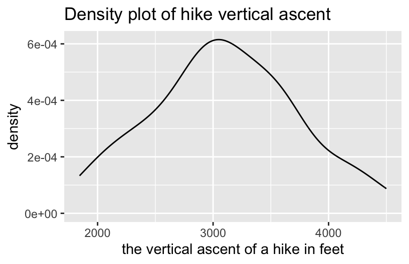
EXAMPLE 4: Wrangling practice – one verb
# How many hikes are in the dataset?


# What's the maximum elevation among the hikes?


# How many hikes are there of each rating?


# What hikes have elevations above 5000 ft?
EXAMPLE 5: Wrangling practice – multiple verbs
# What's the average hike length for each rating category?


# What's the average length of *only* the easy hikes


# What 6 hikes take the longest time to complete?


# What 6 hikes take the longest time per mile?
14.2 Review Handout Part 1: What’s the verb?
Goal: Review some of the functions we’ve learned.
Directions: In your group, complete the provided Part 1 activity. Once you’re done, let me know. I’ll come by to check your answers.
14.3 Review Handout Part 2: Quiz practice
Goal: Practice some problems that are more in the style of the quiz questions. These give you a sense of the structure, vibe, and types of questions that might be asked so that none of that comes as a surprise.
Directions: In your group, complete Part 2 of the activity. Once you’ve completed your work, work on Homework 6 (or anything else related to this class).
14.4 Wrap-up
Quiz 2 is Tuesday. The quiz will cover activities 1-13, as labeled on the online course manual. The exercises will cover a variety of angles. For example…
What does this result mean in context?
You’ll be given some visualization / wrangling results and asked to interpret them.What code is necessary to completing the task at hand?
You’ll be given a task and asked for the necessary code.What does this code do?
You’ll be given some code without output and asked to anticipate the result.
Study tips:
- Make a study sheet based off of the activities. Though you can’t bring this into the quiz, it’s helpful for studying.
- Study your study sheet!
- Review all checkpoints, activities, and homework (in that order). Try doing the exercises without peeking at solutions. Take note of where you need to spend more time studying.
14.5 Solutions
Click for Solutions
EXAMPLE 1: Make a plot
# A boxplot or histogram could also work!
ggplot(hikes, aes(x = ascent)) +
  geom_density()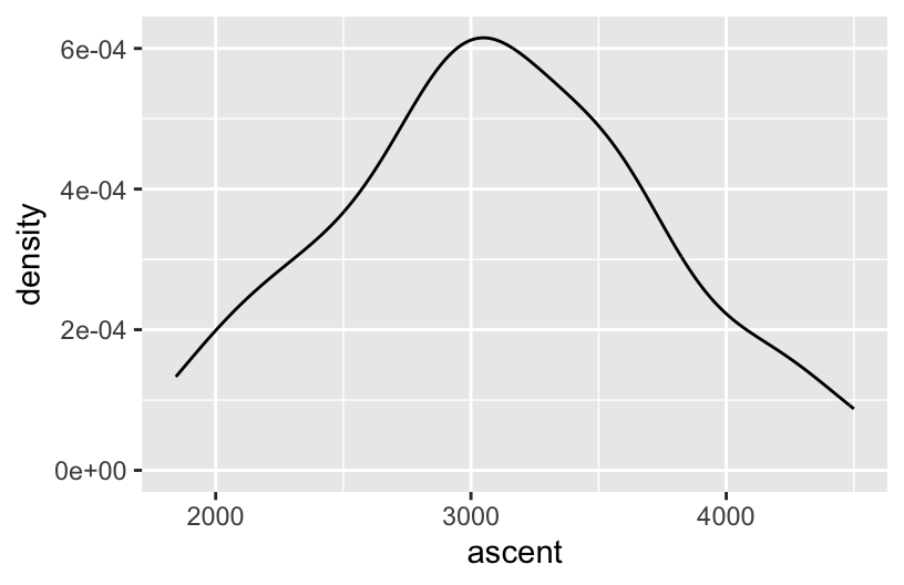
EXAMPLE 2: What’s wrong?
That interpretation doesn’t say anything about the variability in ascent or other important features.
EXAMPLE 3: Captions, axis labels, and titles
The axis label is too long, and the caption and title are redundant.
# Better
ggplot(hikes, aes(x = ascent)) +
  geom_density() +
  labs(x = "vertical ascent (feet)")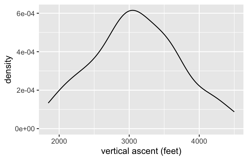
EXAMPLE 4: Wrangling practice – one verb
# How many hikes are in the dataset?
hikes %>%
  nrow()
## [1] 46

# What's the maximum elevation among the hikes?
hikes %>%
  summarize(max(elevation))
##   max(elevation)
## 1           5344

# How many hikes are there of each rating?
hikes %>%
  count(rating)
##      rating  n
## 1 difficult  8
## 2      easy 11
## 3  moderate 27

# What hikes have elevations above 5000 ft?
hikes %>%
  filter(elevation > 5000)
##              peak elevation difficulty ascent length time   rating
## 1     Mt. Marcy        5344          5   3166   14.8   10 moderate
## 2 Algonquin Peak       5114          5   2936    9.6    9 moderate
EXAMPLE 5: Wrangling practice – multiple verbs
# What's the average hike length for each rating category?
hikes %>%
  group_by(rating) %>%
  summarize(mean(length))
## # A tibble: 3 × 2
##   rating    `mean(length)`
##   <chr>              <dbl>
## 1 difficult          17.0
## 2 easy                9.05
## 3 moderate           12.7

# What's the average length of *only* the easy hikes
hikes %>%
  filter(rating == "easy") %>%
  summarize(mean(length))
##   mean(length)
## 1     9.045455

# What 6 hikes take the longest time to complete?
hikes %>%
  arrange(desc(time)) %>%
  head()
##             peak elevation difficulty ascent length time    rating
## 1    Mt. Emmons       4040          7   3490   18.0   18 difficult
## 2   Seward Mtn.       4361          7   3490   16.0   17 difficult
## 3 Mt. Donaldson       4140          7   3490   17.0   17 difficult
## 4  Mt. Skylight       4926          7   4265   17.9   15 difficult
## 5     Gray Peak       4840          7   4178   16.0   14 difficult
## 6  Mt. Redfield       4606          7   3225   17.5   14 difficult

# What 6 hikes take the longest time per mile?
hikes %>%
  mutate(time_per_mile = time / length) %>%
  arrange(desc(time_per_mile)) %>%
  head()
##            peak elevation difficulty ascent length time    rating time_per_mile
## 1   Giant Mtn.       4627          4   3050    6.0  7.5      easy      1.250000
## 2     Nye Mtn.       3895          6   1844    7.5  8.5  moderate      1.133333
## 3  Street Mtn.       4166          6   2115    8.8  9.5  moderate      1.079545
## 4  Seward Mtn.       4361          7   3490   16.0 17.0 difficult      1.062500
## 5    South Dix       4060          6   3050   11.5 12.0  moderate      1.043478
## 6 Cascade Mtn.       4098          2   1940    4.8  5.0      easy      1.041667